Binomial Option Pricing Model: How It Works with Tree Examples

Table of Contents
The binomial option pricing model is one of the most intuitive frameworks for understanding how options are valued. Instead of relying on a complex closed-form equation, the binomial model builds a tree of possible stock prices and works backward from known payoffs at expiration to determine what an option should be worth today. Developed by Cox, Ross, and Rubinstein in 1979, this approach is widely used by quantitative analysts, risk managers, and CFA candidates as the foundation for understanding all option pricing. Whether you’re pricing a simple call option or a complex American put option with early exercise, the binomial model provides a clear, step-by-step framework that connects directly to the option Greeks and more advanced models like Black-Scholes.
What is the Binomial Option Pricing Model?
The binomial option pricing model is a discrete-time model that prices options by constructing a tree of possible stock price movements over multiple time periods. At each step, the stock price can either move up by a factor u or down by a factor d. By starting at expiration (where option payoffs are known) and working backward through the tree, you can calculate the option’s fair value today.
The binomial model’s central insight is that you don’t need to know the actual probability of a stock going up or down to price an option. Instead, it uses risk-neutral probabilities — a mathematical construct where all assets earn the risk-free rate. This no-arbitrage approach produces the same option price regardless of investors’ actual risk preferences.
The model was developed by John Cox, Stephen Ross, and Mark Rubinstein as an intuitive alternative to the Black-Scholes formula. While Black-Scholes provides an elegant closed-form solution for European options, the binomial model offers capabilities the standard closed-form Black-Scholes doesn’t directly provide: a visual, step-by-step framework that can price American options (which allow early exercise), handle discrete dividends, and accommodate changing volatility — making it indispensable for practitioners at investment banks and derivatives desks.
One-Step Binomial Model
The simplest version of the binomial model uses just one time step. A stock currently priced at S can either move up to S × u or down to S × d at expiration. The option’s payoff in each state is known: fu if the stock goes up, and fd if it goes down. The question is: what is the option worth today?
The logic is straightforward: calculate the probability-weighted average of the option’s two possible payoffs (using risk-neutral probability p), then discount that expected value back to today at the risk-free rate. This single formula is the building block for all binomial pricing.
For valid pricing, the model requires d < erΔt < u. This ensures the risk-neutral probability p falls between 0 and 1. If this condition fails — for example, if the risk-free growth exceeds the up factor — arbitrage opportunities exist and the model cannot produce a meaningful price.
Risk-neutral probabilities are not the actual probabilities of the stock going up or down. They are the probabilities that make the expected stock return equal to the risk-free rate — a mathematical construct for no-arbitrage pricing. The real-world probability of an up move is irrelevant for option pricing under this framework.
Multi-Step Binomial Trees
A single time step provides the conceptual foundation, but real-world option pricing requires dividing the option’s life into many smaller steps. In a multi-step binomial tree, each node branches into an up and a down state, creating an expanding lattice of possible stock prices.
CRR Parameters
The most widely used parameterization comes from Cox, Ross, and Rubinstein (CRR). These parameters ensure the binomial tree matches the stock’s observed volatility:
Because d = 1/u, an up move followed by a down move returns the stock to its original price (S × u × d = S). This creates a recombining tree where the number of terminal nodes grows linearly with steps (n + 1 nodes at expiration) rather than exponentially — making computation tractable even for hundreds of steps.
Backward Induction
Once the tree is built forward to expiration, you work backward through it. Starting at the terminal nodes where option payoffs are known, apply the one-step pricing formula at each preceding node to calculate the option value one step earlier. Repeat until you reach the initial node — that’s the option’s fair value today.
A key property: as the number of steps n increases toward infinity, the binomial model converges to the Black-Scholes price for European options. The discrete binomial tree becomes an increasingly fine approximation of the continuous price process that Black-Scholes assumes.
Handling Dividends
For dividend-paying stocks, the binomial model adjusts naturally. With a continuous dividend yield q, the risk-neutral probability becomes:
For discrete dividends, the stock price is reduced at ex-dividend nodes in the tree. This flexibility is a key practical advantage — the binomial model handles dividends more naturally than the standard closed-form Black-Scholes, which requires separate adjustments.
The Replicating Portfolio Approach
There’s an alternative way to derive the binomial option price that provides powerful economic intuition. At each node, you can construct a replicating portfolio consisting of Δ shares of the underlying stock plus B dollars invested in risk-free bonds. If this portfolio has the same payoff as the option in both the up and down states, then by the Law of One Price (no-arbitrage), the portfolio and the option must have the same value.
The hedge ratio Δ tells you exactly how many shares of stock you need to hold to replicate the option. This is the same concept as option delta in the Greeks framework — the binomial model provides an intuitive derivation of why delta equals the ratio of option value changes to stock price changes.
A separate one-period hypothetical example makes replication concrete.
Let the stock start at $100 and finish at either $120 or $80, with a $100
call strike, no dividends and a zero interest rate. The hedge ratio is
Δ = ($20 − $0) / ($120 − $80) = 0.5 shares.
| Position | Today (USD) | Up state: S = $120 (USD) | Down state: S = $80 (USD) |
|---|---|---|---|
| 0.5 shares | 50.00 | 60.00 | 40.00 |
| Borrowing liability | -40.00 | -40.00 | -40.00 |
| Replicating portfolio | 10.00 | 20.00 | 0.00 |
| Call option | 10.00 | 20.00 | 0.00 |
Borrowing $40 finances part of the $50 stock holding. The portfolio
matches the call in both terminal states, fixing today’s call value at
$10 per share under these assumptions.
The replicating portfolio and risk-neutral pricing approaches are two sides of the same coin — they always produce the same option price. The replicating portfolio approach emphasizes the hedging interpretation, while risk-neutral pricing emphasizes the probabilistic interpretation. Use our Delta Hedging Calculator to explore how delta-based hedging works in practice.
Binomial Tree Option Pricing Example
Let’s price a European call option using a 2-step binomial tree. In this hypothetical illustration, a trader evaluates 6-month options on Apple (AAPL) with an assumed stock price of $100 and 20% annualized volatility:
Parameters: Stock price S0 = $100, Strike K = $105, Risk-free rate r = 5%, Volatility σ = 20%, Time to expiration T = 0.5 years, Steps n = 2
Assume no dividends and a continuously compounded annual risk-free rate. Calculations retain full precision; displayed inputs and results are rounded.
Step 1: Calculate Model Inputs
- Δt = T / n = 0.5 / 2 = 0.25 years
- u = eσ√Δt = e0.20 × √0.25 = e0.10 = 1.1052
- d = 1 / u = 0.9048
- p = (erΔt − d) / (u − d) = (1.0126 − 0.9048) / (1.1052 − 0.9048) = 0.5378
Step 2: Build the Stock Price Tree
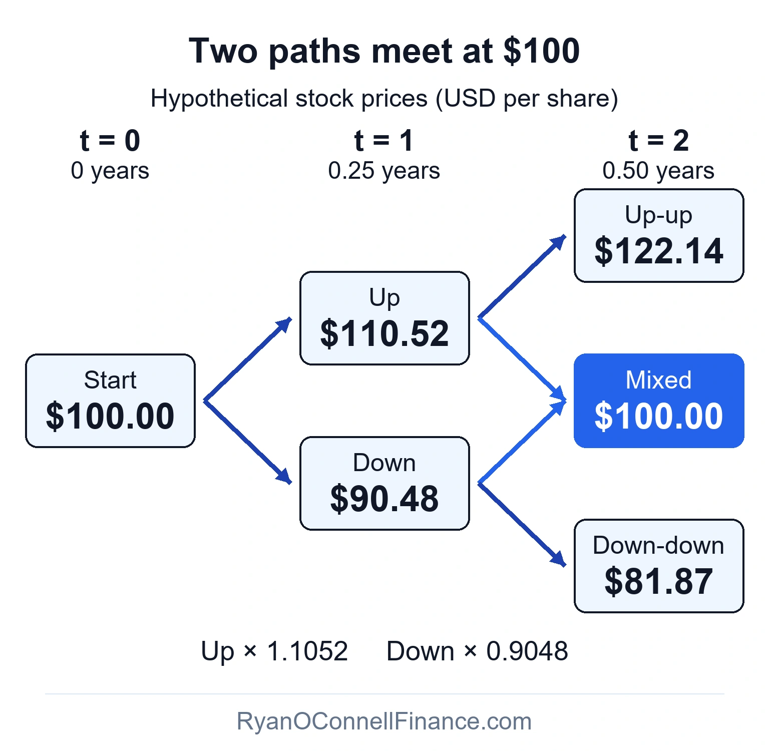
The two mixed paths share one terminal node, so two steps produce three terminal prices rather than four.
Stock prices shown in the tree
| Node | t = 0 | t = 1 | t = 2 |
|---|---|---|---|
| Up-Up | $122.14 | ||
| Up | $110.52 | ||
| Start / Up-Down | $100.00 | $100.00 | |
| Down | $90.48 | ||
| Down-Down | $81.87 |
Step 3: Calculate Call Payoffs at Expiration (K = $105)
- fuu = max($122.14 − $105, 0) = $17.14
- fud = max($100.00 − $105, 0) = $0.00
- fdd = max($81.87 − $105, 0) = $0.00
Step 4: Backward Induction
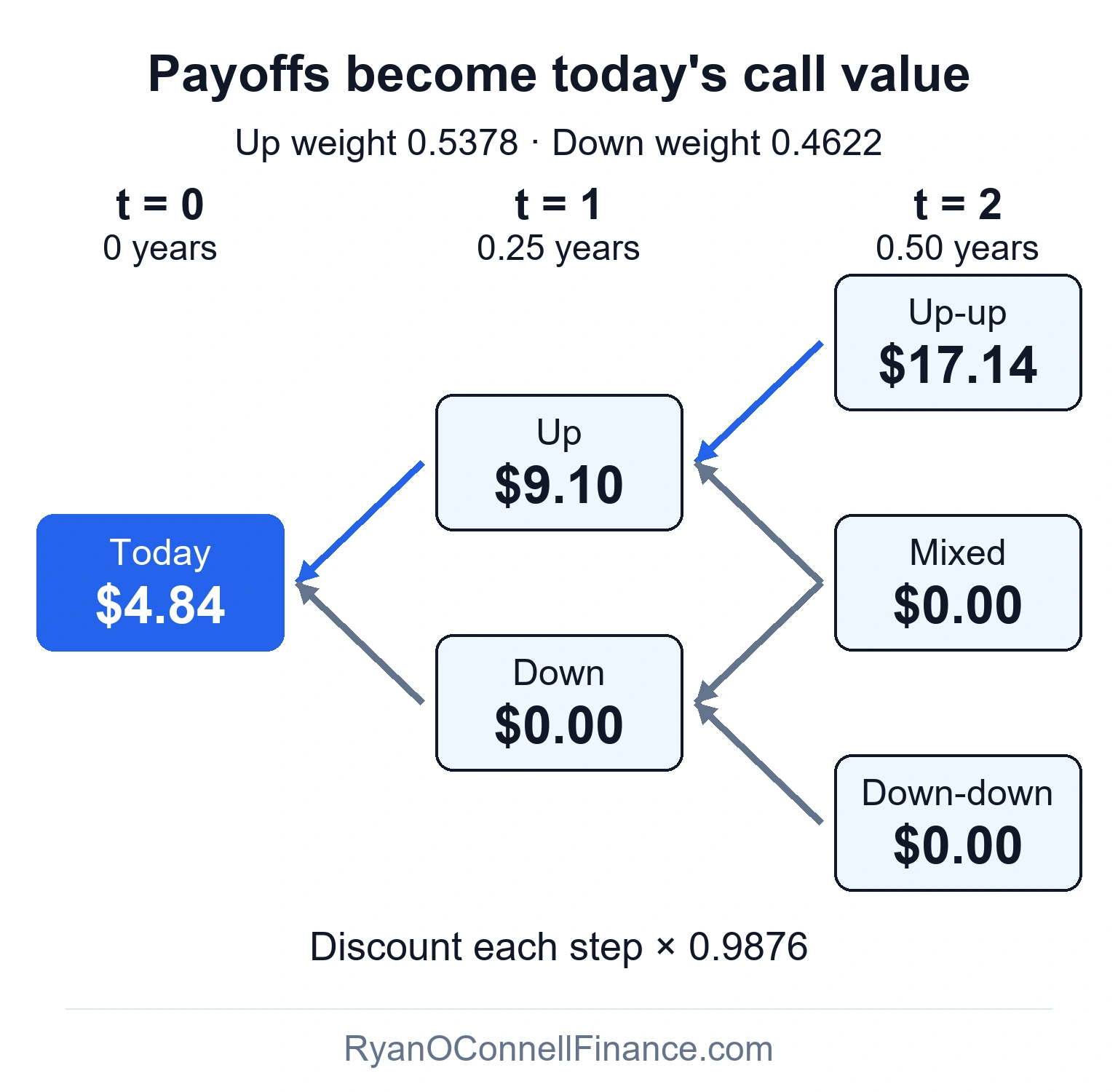
The positive terminal payoff is weighted and discounted twice; the zero-value down branch contributes nothing.
Backward-induction calculations
At t = 1:
- fu ≈ 0.9876 × [0.5378 × $17.1403 + 0.4622 × $0.00] ≈ $9.10
- fd = e−0.0125 × [p × $0.00 + (1 − p) × $0.00] = $0.00
At t = 0:
- f0 ≈ 0.9876 × [0.5378 × $9.1037 + 0.4622 × $0.00] ≈ $4.84
The European call option is worth $4.84.
The replicating portfolio at t = 0 requires Δ = (9.10 − 0.00) / (110.52 − 90.48) = 0.454 shares of stock — illustrating how option delta emerges directly from the binomial framework.
American Options in the Binomial Model
One of the binomial model’s most important advantages over Black-Scholes is its ability to price American options, which can be exercised at any time before expiration. The modification is simple but powerful: at each node during backward induction, compare the continuation value (holding the option) with the exercise value (exercising immediately), and take the maximum.
An important nuance: for American call options on non-dividend-paying stocks, under the standard frictionless model with nonnegative interest rates, early exercise offers no advantage over holding the call. Its value is at least its immediate exercise value; strict positive time value is not universal. Early exercise is primarily relevant for American put options (which may be exercised early when deep in-the-money) and for calls on dividend-paying stocks (where exercising just before an ex-dividend date can be optimal).
Using the same hypothetical, no-dividend parameters — imagine a portfolio manager holding protective puts on General Electric (GE) at S0 = $100, K = $105, r = 5%, σ = 20%, T = 0.5yr, 2-step tree — let’s price an American put option:
Put Payoffs at Expiration (K = $105)
- guu = max($105 − $122.14, 0) = $0.00
- gud = max($105 − $100.00, 0) = $5.00
- gdd = max($105 − $81.87, 0) = $23.13
Backward Induction with Early Exercise Check
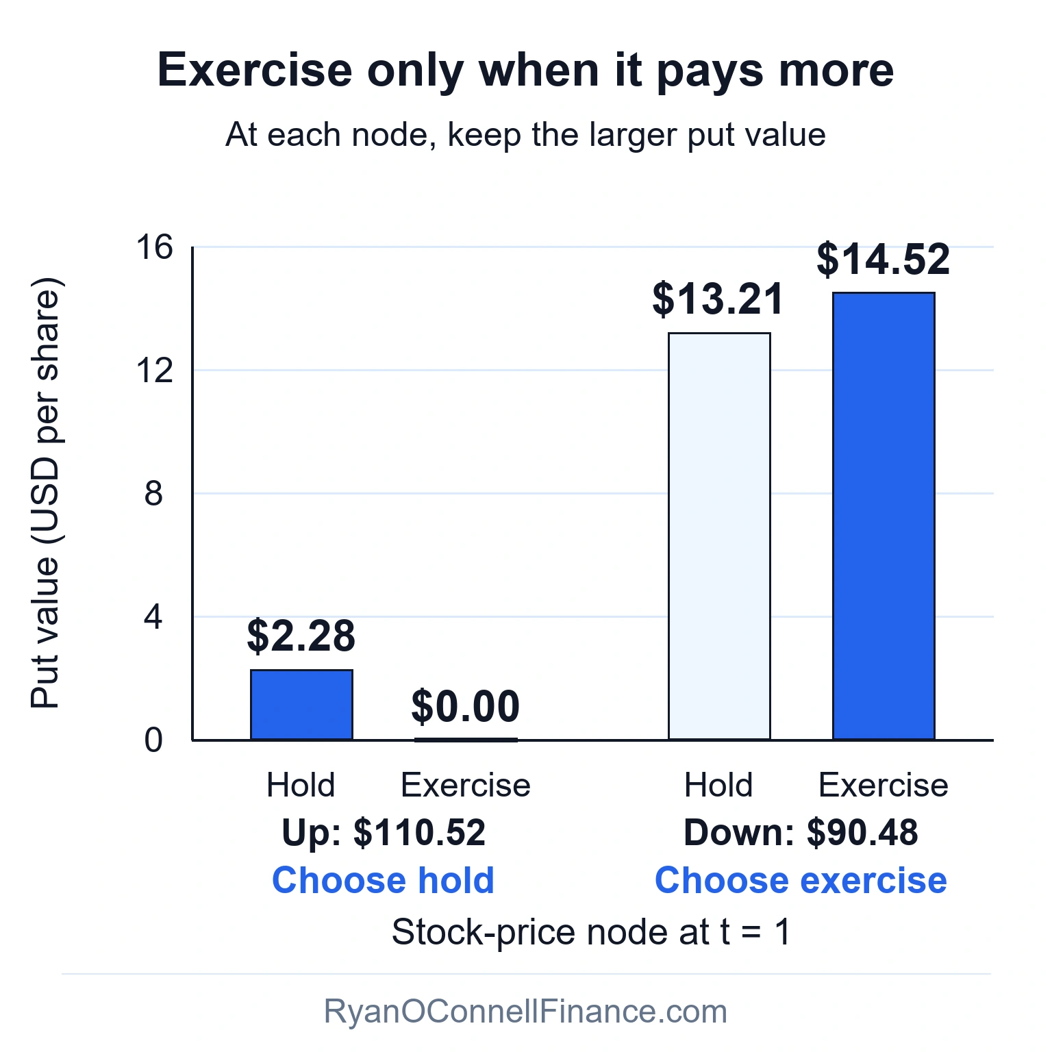
Holding wins at the up node. At the down node, exercising adds about $1.30 per share over continuation.
Early-exercise calculations
At t = 1, Up node (S = $110.52):
- Continuation value = 0.9876 × [0.5378 × $0.00 + 0.4622 × $5.00] = $2.28
- Exercise value = max($105 − $110.52, 0) = $0.00
- Decision: Continue holding ($2.28 > $0.00)
At t = 1, Down node (S = $90.48):
- Continuation value = 0.9876 × [0.5378 × $5.00 + 0.4622 × $23.13] = $13.21
- Exercise value = max($105 − $90.48, 0) = $14.52
- Decision: Exercise early! ($14.52 > $13.21)
At t = 0:
- g0 = 0.9876 × [0.5378 × $2.28 + 0.4622 × $14.52] = $7.84
- Exercise value = max($105 − $100, 0) = $5.00 < $7.84 → Continue holding
American put value = $7.84 vs. European put value = $7.24
The early exercise premium is $0.60 — this is the additional value from having the right to exercise before expiration. At the down node, the put is deep in-the-money and the intrinsic value ($14.52) exceeds the continuation value ($13.21), making immediate exercise optimal.
Binomial Model vs Black-Scholes
The binomial model and Black-Scholes are the two foundational approaches to option pricing. Understanding when to use each is essential for practitioners and students alike.
Binomial Model
- Discrete time steps — prices at specific intervals
- Handles American options with early exercise check at every node
- Visual and intuitive — tree provides node-level insight into exercise decisions
- Flexible — naturally accommodates dividends and changing volatility
- Computationally intensive for many steps
Black-Scholes Model
- Continuous time — elegant closed-form formula
- Closed-form solution applies to European options (approximations exist for some American cases)
- Faster computation — single formula evaluation
- Assumes constant volatility and continuous trading
- Less flexible with dividends (requires separate adjustments)
In practice, the two models are complementary. As the number of binomial steps increases, the binomial price converges to the Black-Scholes price for European options — the binomial tree is a discrete approximation of the continuous process Black-Scholes assumes. For American options, exotic structures, or situations with discrete dividends, the binomial model is often the preferred approach. For quick European option pricing under standard assumptions, Black-Scholes is faster and more convenient.
How to Price Options Using the Binomial Model
Here is the complete step-by-step process for pricing any option using the binomial model:
- Define parameters: Identify the stock price (S), strike price (K), risk-free rate (r), volatility (σ), time to expiration (T), and number of steps (n)
- Calculate CRR inputs: Compute Δt = T/n, then u = eσ√Δt, d = 1/u, and p = (erΔt − d) / (u − d)
- Verify no-arbitrage: Confirm d < erΔt < u (equivalently, 0 < p < 1)
- Build the stock price tree: Starting from S0, multiply by u for up moves and d for down moves at each step
- Calculate terminal payoffs: At expiration, compute max(S − K, 0) for calls or max(K − S, 0) for puts
- Work backward: At each node, apply f = e−rΔt × [p × fu + (1 − p) × fd]
- For American options: At every node, compare the continuation value with the exercise value and take the maximum
In practice, 50–100 steps produce prices very close to Black-Scholes for European options. For American options, 200+ steps may be needed for high precision.
Common Mistakes
The binomial model is conceptually straightforward, but several common errors can lead to incorrect option prices:
1. Using real-world probabilities instead of risk-neutral probabilities. The binomial model uses risk-neutral probabilities (p), not the actual probability of a stock going up. Real-world probabilities reflect investor expectations; risk-neutral probabilities are a mathematical construct for no-arbitrage pricing. Using real-world probabilities produces incorrect option values.
2. Forgetting to discount during backward induction. Each backward step requires multiplying by the discount factor e−rΔt. Omitting this factor overstates the option value because it ignores the time value of money.
3. Using incorrect u and d parameters. A common error is using u = 1 + σ instead of the correct CRR formula u = eσ√Δt. The simplified version doesn’t properly capture the stock’s volatility dynamics and produces wrong tree structures.
4. Not checking early exercise for American options. The binomial model’s key advantage is pricing American options, but you must explicitly compare the continuation value with the exercise value at every node. Skipping this check treats the American option as European and undervalues it.
5. Confusing up/down factors with probabilities. The up factor u and down factor d are price multipliers that determine how much the stock moves. The risk-neutral probability p determines the weighting in the expected payoff calculation. These serve fundamentally different roles in the model.
6. Mixing annualized and per-step inputs. Volatility σ and the risk-free rate r are quoted as annualized figures, but the model uses per-step values (σ√Δt and rΔt). Forgetting to scale inputs by the step size Δt produces wrong u, d, and p values.
7. Not verifying the no-arbitrage condition. If the computed risk-neutral probability p falls outside the range [0, 1], the parameters are inconsistent — typically because the step size Δt is too large relative to the volatility. This signals bad parameterization: reduce Δt (increase the number of steps) or check your inputs.
Limitations of the Binomial Model
The binomial model is an approximation — it discretizes what is really a continuous price process. While it converges to Black-Scholes as the number of steps increases, trees with few steps can produce less accurate prices with step-like behavior in the pricing function.
1. Computational intensity. Although recombining trees reduce the number of terminal nodes at maturity from 2n to just n + 1, pricing still requires visiting every node in the tree. For very large trees or when pricing many options simultaneously, computation time can become significant.
2. Constant volatility assumption. The standard binomial model uses the same volatility σ at every node. In reality, implied volatility varies across strike prices (the volatility smile) and over time (the term structure of volatility). Extensions exist to address this, but they add complexity.
3. Parameter sensitivity. Small changes in volatility or the risk-free rate can meaningfully change the computed option price, especially for options near the money or close to expiration. Practitioners should test sensitivity to input parameters.
4. Discrete approximation artifacts. With few steps, the binomial price can oscillate as you change n (odd vs. even step counts can give different convergence behavior). Using Richardson extrapolation or averaging odd/even results can mitigate this issue.
| Tree steps (n) | CRR | Black-Scholes |
|---|---|---|
| 2 | 4.84 | 4.58 |
| 3 | 4.68 | 4.58 |
| 4 | 4.83 | 4.58 |
| 5 | 4.50 | 4.58 |
| 6 | 4.78 | 4.58 |
| 7 | 4.43 | 4.58 |
| 8 | 4.74 | 4.58 |
| 9 | 4.43 | 4.58 |
| 10 | 4.71 | 4.58 |
| 11 | 4.51 | 4.58 |
| 12 | 4.68 | 4.58 |
| 13 | 4.55 | 4.58 |
| 14 | 4.66 | 4.58 |
| 15 | 4.58 | 4.58 |
| 16 | 4.64 | 4.58 |
| 17 | 4.60 | 4.58 |
| 18 | 4.62 | 4.58 |
| 19 | 4.61 | 4.58 |
| 20 | 4.60 | 4.58 |
| 21 | 4.62 | 4.58 |
| 22 | 4.59 | 4.58 |
| 23 | 4.62 | 4.58 |
| 24 | 4.58 | 4.58 |
| 25 | 4.62 | 4.58 |
| 26 | 4.57 | 4.58 |
| 27 | 4.62 | 4.58 |
| 28 | 4.56 | 4.58 |
| 29 | 4.62 | 4.58 |
| 30 | 4.55 | 4.58 |
| 31 | 4.62 | 4.58 |
| 32 | 4.54 | 4.58 |
| 33 | 4.62 | 4.58 |
| 34 | 4.54 | 4.58 |
| 35 | 4.62 | 4.58 |
| 36 | 4.55 | 4.58 |
| 37 | 4.61 | 4.58 |
| 38 | 4.56 | 4.58 |
| 39 | 4.61 | 4.58 |
| 40 | 4.57 | 4.58 |
Hypothetical European call: S = $100, K = $105, r = 5%, σ = 20%, T = 0.5 years; no dividends. Values rounded to cents.
For these inputs, two steps give $4.84 and 40 steps give $4.57,
compared with $4.58 from Black-Scholes. The swings narrow, but accuracy
does not improve with every additional step.
Despite these limitations, the binomial model remains one of the most widely taught and practically useful option pricing frameworks. Its transparency, flexibility, and convergence to Black-Scholes make it an essential tool for anyone working with options.
Frequently Asked Questions
Disclaimer
This article is for educational and informational purposes only and does not constitute investment advice. Option pricing models involve simplifying assumptions that may not reflect actual market conditions. Example calculations use hypothetical parameters for illustration. Always conduct your own research and consult a qualified financial advisor before making investment decisions. See also our articles on put-call parity for the fundamental relationship between call and put prices.
Keep reading
Next in this series
Part 2 of 3 in Option Pricing Models
Put-Call Parity: Formula, Arbitrage, and Synthetic Positions ExplainedMore in Options & Derivatives
-
Call Options: Buying and Selling Calls Explained
Complete guide to call options — how they work, buying vs selling calls, payoff diagrams, and when to use call options in your trading strategy.
-
Put Options: Buying and Selling Puts Explained
Complete guide to put options — how they work, buying vs selling puts, payoff diagrams, hedging applications, and when to use put options.
-
Option Greeks: The Complete Beginner’s Guide
Complete guide to the five option Greeks — delta, gamma, theta, vega, and rho — what they measure, how they interact, and how to use them for options analysis.