Deadweight Loss & the Costs of Taxation

Table of Contents
Deadweight loss is one of the most important concepts in economics for understanding why taxes impose costs beyond the revenue they raise. Every per-unit tax drives a wedge between what buyers pay and what sellers receive, shrinking markets below their efficient size and destroying consumer and producer surplus that no one captures. While deadweight loss can also arise from price controls, quotas, monopoly pricing, and subsidies, this article focuses on taxation — how taxes create deadweight loss, why elasticity determines its size, and the trade-off between government revenue and economic efficiency.
What is Deadweight Loss?
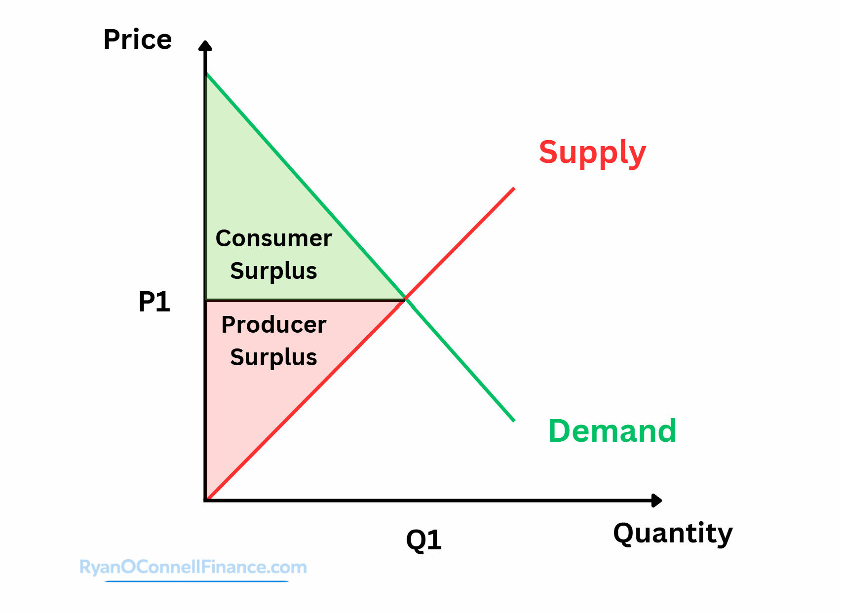
In a free market, buyers and sellers trade until the marginal benefit of the last unit sold equals its marginal cost. At this equilibrium quantity, total surplus — the combined gains to buyers and sellers — is maximized. When a tax is imposed, some trades that would benefit both parties no longer occur because the tax makes them unprofitable.
Deadweight loss is the reduction in total surplus that results when a tax shrinks a market below its efficient level. It represents the value of mutually beneficial trades that no longer happen — losses to buyers and sellers that are not offset by government tax revenue.
Consider a simple example from economist N. Gregory Mankiw. Jane values having her house cleaned at $120. Joe’s opportunity cost of cleaning it is $80. Without a tax, they trade at $100 — Jane gains $20 of consumer surplus, Joe gains $20 of producer surplus, and total surplus is $40. Now suppose the government imposes a $50 tax on cleaning services. The tax exceeds the $40 of total surplus the trade generates, so the trade never happens. Jane doesn’t get her house cleaned, Joe doesn’t earn the income, and the government collects nothing. That $40 of destroyed surplus is pure deadweight loss.
Deadweight Loss on a Supply and Demand Graph
On a supply and demand graph, a tax creates a tax wedge — a gap between the price buyers pay (PB) and the price sellers receive (PS), where PB – PS equals the tax amount. This wedge causes the quantity traded to fall from Q1 (the free-market equilibrium) to Q2 (the post-tax quantity).
The welfare effects of a tax can be traced using the areas on the graph:
| Measure | Without Tax | With Tax | Change |
|---|---|---|---|
| Consumer Surplus | A + B + C | A | Falls by B + C |
| Producer Surplus | D + E + F | F | Falls by D + E |
| Tax Revenue | 0 | B + D | Rises by B + D |
| Total Surplus | A + B + C + D + E + F | A + B + D + F | Falls by C + E |
The areas B and D are transferred from buyers and sellers to the government as tax revenue — a redistribution, not a loss. But areas C and E form the deadweight loss triangle: the surplus that vanishes entirely because those units are no longer traded. The triangle sits between the supply and demand curves, bounded horizontally by Q2 and Q1, with its height equal to the tax wedge.
In the standard competitive model, a tax on a good produces the same market outcome regardless of whether it is legally imposed on buyers or sellers. The tax wedge, equilibrium quantities, and deadweight loss are identical in both cases. Who truly bears the burden depends on elasticity, not on who writes the check to the government.
How to Calculate Deadweight Loss
Because the deadweight loss region forms a triangle on the supply and demand graph, its area can be calculated using a simple formula:
Where ΔQ = Q1 – Q2, the number of units that are no longer traded after the tax is imposed. The government collects tax revenue on the units still traded:
A critical insight is how deadweight loss scales with the size of the tax. In a standard linear partial-equilibrium model, both the base and the height of the deadweight loss triangle grow with the tax, so deadweight loss increases with the square of the tax rate:
Because deadweight loss grows with the square of the tax rate, policymakers can minimize total economic distortion by applying broad-based taxes at low rates rather than narrow taxes at high rates. A 5% tax on everything creates far less deadweight loss than a 50% tax on one good.
Who Bears the Burden of a Tax?
Tax incidence describes how the economic burden of a tax is divided between buyers and sellers. The key insight is that the less elastic side of the market bears more of the tax burden, because they have fewer alternatives and cannot easily change their behavior to avoid the tax. At the same time, more elastic supply and demand creates more deadweight loss, because quantity responds more sharply to the tax wedge.
The U.S. payroll tax (FICA) is legally split 50/50 between employers and employees — each pays 7.65% of wages. Congress designed this split to share the burden equally. However, labor economists find that labor supply is often less elastic than labor demand — workers have fewer alternatives than firms do when it comes to adjusting behavior. As a result, workers often bear most of the payroll tax burden in the form of lower pre-tax wages, regardless of the legal split.
The lesson: Lawmakers can decide who writes the check to the government, but market forces — specifically, relative elasticities — decide who truly pays.
The Luxury Tax of 1990 provides another instructive case. Congress imposed excise taxes on yachts, private airplanes, furs, jewelry, and expensive automobiles, reasoning that only the wealthy bought these goods. But demand for luxury goods is highly elastic — the rich have many alternatives and can simply postpone purchases. Supply, on the other hand, is relatively inelastic in the short run — boat factories and skilled workers cannot easily switch to other industries. The burden fell primarily on middle-class workers who built yachts, not on wealthy buyers. Most of these luxury excise taxes were repealed in 1993; the automobile tax was modified rather than eliminated outright.
Elasticity and Deadweight Loss
The size of the deadweight loss from a tax depends on how much buyers and sellers change their behavior in response to the price change. The more elastic supply and demand are, the more quantity falls, and the larger the deadweight loss triangle becomes.
| Scenario | Supply Elasticity | Demand Elasticity | DWL Size | Why |
|---|---|---|---|---|
| Both inelastic | Low | Low | Small | Neither side changes behavior much; quantity barely falls |
| Elastic supply, inelastic demand | High | Low | Medium | Sellers exit the market, but buyers keep purchasing |
| Inelastic supply, elastic demand | Low | High | Medium | Buyers cut back sharply, but sellers remain |
| Both elastic | High | High | Large | Both sides adjust sharply; quantity drops dramatically |
From an efficiency perspective — holding equity and externality considerations constant — economists generally prefer taxing goods with inelastic demand (such as gasoline, tobacco, or prescription medications). When buyers and sellers cannot easily change their behavior, the tax raises revenue with minimal deadweight loss. For more on measuring responsiveness to price changes, see our guide to price elasticity of demand.
Deadweight Loss Example: Gasoline Tax
The following stylized example illustrates how to compute deadweight loss and tax revenue from an excise tax.
Setup: In a hypothetical market, gasoline trades at a pre-tax equilibrium price of $3.00 per gallon with a quantity of 400 million gallons per month. The government imposes a $2.00 per gallon excise tax.
| Variable | Value |
|---|---|
| Pre-tax price | $3.00/gallon |
| Pre-tax quantity | 400 million gallons/month |
| Tax per gallon | $2.00 |
| Post-tax buyer price (PB) | $3.80 |
| Post-tax seller price (PS) | $1.80 |
| Post-tax quantity (Q2) | 340 million gallons/month |
Tax incidence: Buyers pay $0.80 more per gallon (40% of the tax). Sellers receive $1.20 less per gallon (60% of the tax). Sellers bear a larger share because, in this example, gasoline supply is less elastic than demand, so sellers are less able than buyers to adjust quantity in response to the tax.
Deadweight loss: DWL = ½ × $2.00 × 60 million = $60 million per month
Tax revenue: $2.00 × 340 million = $680 million per month
Scaling illustration: If the tax doubled to $4.00 per gallon, deadweight loss would roughly quadruple to approximately $240 million per month — not just double — because both the base and height of the DWL triangle expand with the tax.
Deadweight Loss vs. Tax Revenue: The Laffer Curve
The Laffer curve illustrates the relationship between tax rates and government revenue. At a 0% tax rate, the government collects no revenue. At a 100% tax rate, no one would produce or trade, so revenue is again zero. Revenue is maximized somewhere in between — but that revenue-maximizing rate is not the same as the welfare-maximizing rate, because deadweight loss continues to grow even after revenue peaks.
Economist Arthur Laffer famously sketched this curve on a napkin in 1974 during a dinner with journalists and political advisors. The concept influenced President Reagan’s supply-side economics platform, which argued that U.S. tax rates were on the downward-sloping portion of the curve — so tax rate cuts would actually increase revenue. Most economists remain skeptical that the U.S. was on that portion of the curve, though the theoretical relationship itself is uncontested.
Low Tax Rates
- Small tax wedge
- Minimal behavioral distortion
- Most beneficial trades still occur
- Revenue grows as rate increases
- Deadweight loss is small
Revenue-Maximizing Rate
- Optimal balance between rate and base
- Moderate behavioral distortion
- Tax base still large enough for peak revenue
- Deadweight loss is significant
- Further rate increases reduce revenue
High Tax Rates
- Large tax wedge shrinks market sharply
- Many trades no longer occur
- Tax base shrinks faster than rate grows
- Revenue falling despite higher rate
- DWL grows with the square of the tax
Prohibitive Rate (100%)
- No voluntary market activity occurs
- Tax revenue drops to zero
- Maximum deadweight loss
- All gains from trade destroyed
- Extreme case — theoretical limit
Economists broadly agree that the Laffer curve is theoretically valid, but they remain divided on where any particular economy sits on the curve. The revenue-maximizing tax rate depends on the specific market, time period, and behavioral elasticities involved — it is an empirical question, not a fixed number.
Common Mistakes
Deadweight loss and tax incidence are frequently misunderstood. Here are the most common errors:
1. Confusing who writes the check with who bears the burden. Many people assume that if a tax is levied on sellers, sellers pay the full amount. In reality, the economic burden depends on the relative price elasticity of demand and supply, not on who is legally responsible for remitting the tax.
2. Thinking deadweight loss equals the entire tax amount. Tax revenue (the rectangle on the graph) is a transfer from buyers and sellers to the government — a redistribution, not a net loss to society. Deadweight loss is only the triangle of surplus destroyed by trades that no longer happen. It is always smaller than total tax revenue unless the tax is so high it nearly destroys the market.
3. Assuming deadweight loss doubles when the tax doubles. Because DWL is proportional to the square of the tax in standard linear models, doubling a tax roughly quadruples the deadweight loss. This is one of the most counterintuitive — and most important — results in tax economics.
4. Ignoring what the government does with tax revenue. Deadweight loss analysis measures only the efficiency cost of market distortion. If the government uses revenue for public goods that generate large social benefits (infrastructure, national defense, education), the net welfare effect of the tax may be positive even though deadweight loss exists.
5. Thinking the side that bears more tax burden also creates more deadweight loss. Tax incidence and deadweight loss are driven by different mechanics. The less elastic side absorbs more of the tax burden (because it cannot adjust behavior to avoid the tax), while more elastic markets produce larger deadweight loss (because quantity responds more sharply). These are distinct concepts that often move in opposite directions.
Limitations
The standard deadweight loss analysis assumes perfectly competitive markets, rational actors, and no externalities. In markets where these assumptions fail, the conclusions may differ significantly from the textbook model.
Externalities change the calculus. If a good produces negative externalities (pollution, congestion, secondhand smoke), the free-market equilibrium is not truly efficient. A Pigouvian tax that corrects for the externality can actually increase total welfare, even though it creates a measured deadweight loss in the taxed market. A carbon tax, for example, may improve overall efficiency by forcing producers to internalize environmental costs.
Administrative and compliance costs are excluded. The deadweight loss triangle captures only the distortion from changed behavior. It ignores the real resources spent on tax compliance — accountants, lawyers, record-keeping — and tax administration, which are also genuine costs of taxation.
The analysis assumes static partial equilibrium. Standard DWL calculations examine one market in isolation. In reality, taxes in one market cause substitution effects that ripple across other markets. General equilibrium effects can amplify or offset the measured deadweight loss.
Elasticity estimates are debated. Calculating deadweight loss requires knowing how much quantity changes in response to a tax, which depends on accurate elasticity estimates. These estimates vary across studies and are a major source of disagreement in policy debates — the labor supply elasticity debate, for instance, underlies much of the controversy over income tax policy. For how price ceilings and price floors create deadweight loss through different mechanisms, see our dedicated guide.
Frequently Asked Questions
Disclaimer
This article is for educational and informational purposes only and does not constitute financial, tax, or legal advice. Tax incidence and deadweight loss calculations presented here are simplified illustrations based on standard economic models. Actual tax effects depend on market conditions, regulatory frameworks, and behavioral responses that may differ from theoretical predictions. Consult a qualified tax professional for guidance on specific tax situations.


