Enter Values

Enter as decimal (e.g., 0.75 means 75% of income is spent)
$ B
Positive = spending increase, Negative = spending decrease
%
0% = no crowding out, 100% = complete crowding out
Shows how spending cascades through the economy
Multiplier Formulas
Spending: 1 / (1 − MPC)
Tax: −MPC / (1 − MPC)
Balanced Budget: = 1 (always)
MPC = Marginal Propensity to Consume | MPS = 1 − MPC
Ryan O'Connell, CFA
Calculator by Ryan O'Connell, CFA

Calculation Result

Total GDP Change (ΔY) $400.0B Expansionary
MPS 0.25
Spending Mult. 4.00
Tax Mult. -3.00
BBM 1.00
Effective Multiplier --
Adjusted ΔY --
Balanced-Budget Multiplier = 1: An equal increase in government spending and lump-sum taxes raises GDP by exactly the amount of the policy change, regardless of MPC.

Formula Breakdown

Spending Multiplier = 1 / (1 − MPC)
Step-by-step calculation for your selected policy type

Spending Rounds

Round New Spending Cumulative

Balanced-Budget Multiplier = 1

The spending increase and tax increase have opposing multiplier effects that largely cancel. The net result is that GDP rises by exactly the amount of the policy change, with no additional multiplier amplification. The spending rounds table does not apply in this mode.

Model Assumptions
  • Simple Keynesian cross model (fixed price level, no supply constraints)
  • MPC is constant across all income levels and spending rounds
  • Closed economy — no import leakage (open-economy multipliers are smaller)
  • Crowding out modeled as a simplified percentage reduction, not derived from IS-LM
  • Tax multiplier assumes lump-sum taxes (not marginal rate changes or endogenous taxes)
  • Balanced-budget multiplier = 1 assumes simultaneous equal changes in G and lump-sum T
  • Does not account for Ricardian equivalence, implementation lags, or supply-side effects

For educational purposes. Not financial advice. Market conventions simplified.

Understanding the Fiscal Multiplier

What is the Fiscal Multiplier?

The fiscal multiplier measures how much total GDP changes in response to a change in government spending or taxes. In the simple Keynesian cross model, when the government spends $1, that dollar becomes income for someone — a worker, a supplier, or a business owner. That person then spends a fraction of that new income (determined by their MPC), which becomes income for someone else, creating a cascading chain of spending.

With an MPC of 0.75, each $1 of government spending eventually generates $4 of total GDP through this multiplier process. The formula is straightforward: Multiplier = 1 / (1 − MPC) = 1 / MPS.

Key Multiplier Formulas
Spending: 1 / (1 − MPC) = 1 / MPS
Tax: −MPC / (1 − MPC) = −MPC / MPS
Balanced Budget: Always = 1
Based on Mankiw, Chapter 21 (Sections 21.2–21.3)

Spending Multiplier vs. Tax Multiplier

Spending Multiplier

1 / MPS
Government purchases enter demand dollar-for-dollar in Round 1. The full $1 becomes new spending immediately, maximizing the cascade effect.

Tax Multiplier

−MPC / MPS
A tax cut increases disposable income, but households save (1 − MPC) of it. Only MPC × $1 enters spending in Round 1, making the absolute effect smaller.

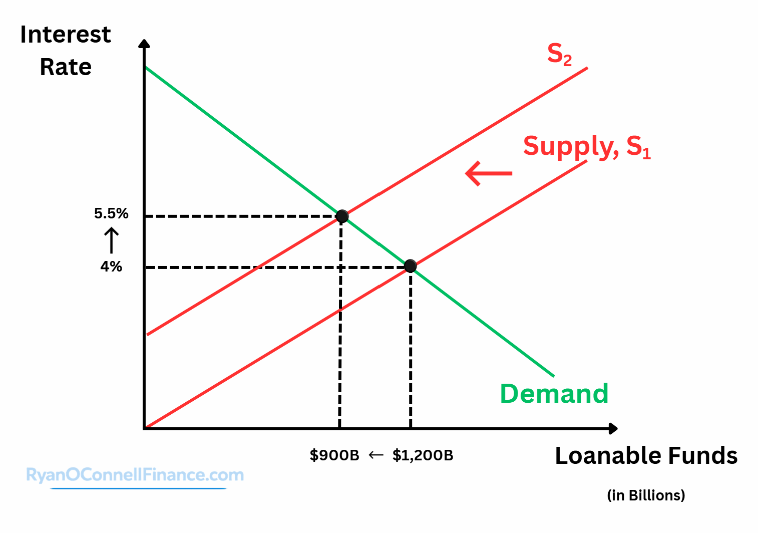
The Crowding-Out Effect

When the government increases spending financed by borrowing, it increases demand for loanable funds, which pushes up interest rates. Higher interest rates make borrowing more expensive for businesses and households, reducing private investment spending. This crowding-out effect partially offsets the multiplier’s stimulus.

This calculator models crowding out as a simple percentage reduction — a heuristic approximation. In practice, the magnitude depends on monetary policy response, the state of the economy, and financial market conditions.

Crowding-out effect: government borrowing shifts loanable funds supply left (S1 to S2), raising interest rates from 4% to 5.5% and reducing funds from $1,200B to $900B
Figure: When the government borrows to finance spending, the supply of loanable funds shifts left (S1 → S2), pushing interest rates up (4% → 5.5%) and reducing private investment ($1,200B → $900B). This crowding-out effect partially offsets fiscal stimulus.
Important: The simple Keynesian multiplier model assumes a closed economy with fixed prices. Real-world multipliers are affected by import leakage, inflation responses, monetary policy offsets, and consumer expectations about future taxes (Ricardian equivalence).

Key Model Limitations

  • Fixed price level — no inflation response to demand changes
  • Closed economy — no import leakage (open-economy multipliers are smaller)
  • Constant MPC across income levels and rounds
  • Tax multiplier uses lump-sum taxes only (not marginal rate changes)
  • No Ricardian equivalence — consumers don’t offset government borrowing
  • No implementation lags or supply-side constraints

Frequently Asked Questions

The fiscal multiplier measures how much GDP changes for each dollar of government spending change. When the government spends $1, that becomes income for someone who then spends MPC of it, creating a chain reaction. With MPC = 0.75, each $1 of spending eventually generates $4 of GDP (multiplier = 1/(1-0.75) = 4). The process works through successive rounds: Round 1 = $1, Round 2 = $0.75, Round 3 = $0.5625, and so on, converging to $4 total.

MPC is the fraction of each additional dollar of income that households spend on consumption rather than save. If MPC = 0.75, households spend 75 cents and save 25 cents of each extra dollar. The marginal propensity to save (MPS) is 1 − MPC. MPC determines the multiplier's size — higher MPC means a larger multiplier because more income recirculates through the economy.

A $1 government purchase directly becomes $1 of new spending in Round 1 — the full dollar enters aggregate demand immediately. A $1 tax cut gives households an extra dollar, but they only spend MPC of it (saving the rest). So the first-round demand impact of a tax cut is MPC × $1, which is less than $1. This initial leakage to saving makes the tax multiplier (−MPC/MPS) smaller in absolute value than the spending multiplier (1/MPS). For example, with MPC = 0.75: spending multiplier = 4, tax multiplier = −3.

The balanced-budget multiplier applies when government increases spending and lump-sum taxes by the same amount simultaneously. Algebraically: BBM = Spending Multiplier + Tax Multiplier = 1/MPS + (−MPC/MPS) = (1 − MPC)/MPS = MPS/MPS = 1. So a $20B increase in both G and T raises GDP by exactly $20B, regardless of MPC. This assumes equal simultaneous changes and lump-sum taxes with no endogenous offsets.

When government borrowing increases to fund spending, it raises demand for loanable funds, pushing up interest rates. Higher interest rates reduce private investment spending, partially offsetting the fiscal stimulus. This calculator uses a simplified percentage reduction to model crowding out — it is not derived from a full IS-LM model. The actual magnitude depends on monetary policy response, economic slack, and financial conditions. In balanced-budget mode, crowding out is hidden because the spending is tax-financed rather than deficit-financed.

The model assumes: (a) fixed price level (no inflation response), (b) closed economy (no import leakage), (c) constant MPC across all income levels, (d) no Ricardian equivalence (consumers don't offset government borrowing by saving more), (e) no implementation lags, and (f) no supply-side constraints. The tax multiplier specifically assumes lump-sum taxes, not marginal rate changes. Real-world multipliers are typically smaller than the simple formula suggests, especially when the economy is near full capacity.
Disclaimer

This calculator is for educational purposes only and uses the simple Keynesian cross model with fixed prices, constant MPC, and a closed economy. Real-world fiscal multipliers depend on monetary policy, economic conditions, trade openness, and consumer expectations. This tool should not be used for policy recommendations.