Correlation Explained

Table of Contents
Correlation helps answer a useful investing question: do two holdings tend to do better
and worse than usual at the same time? This matters when assessing
portfolio diversification, which spreads money
across investments that may perform differently.[6]
A correlation coefficient condenses one aspect of that relationship into a number.
Understanding the number starts with looking at the observations behind it.
What Is Correlation?
Pearson correlation, usually written r for a sample,
measures the direction and strength of the linear relationship between
two numerical variables. Its value runs from −1 to +1 when both variables have
nonzero variation.[1]
The sign tells you the direction of the straight-line pattern. The distance from
zero tells you its strength. A coefficient near zero can still accompany a clear
curved relationship.[4]
The video gives a visual introduction. The worked example below uses its own
clearly hypothetical returns so you can check the calculation independently.
Start With a Scatterplot
Suppose you want to compare the daily price moves of Coca-Cola and PepsiCo.
First express each move as a return. A hypothetical increase from $100 to $102 gives
($102 − $100) / $100 = 0.02 = 2%. This simple price return
measures the price change; it excludes dividends.
Pair the two returns from each matching trading day. Put Coca-Cola’s return on
the horizontal axis and PepsiCo’s on the vertical axis. Each day’s pair becomes
one dot. A scatterplot shows the corresponding values of two variables and helps
reveal their relationship.[3]
- Direction: Does the cloud tilt upward or downward?
- Form: Does it follow a straight line, a curve, or no clear pattern?
- Strength: How tightly do the dots cluster around the pattern?
- Unusual points: Are any observations far from the rest?
For another investing question, you could pair Apple’s daily returns with the
S&P 500’s daily returns to examine their linear association. Either comparison
needs matching periods and a clearly defined return measure. The
descriptive statistics of each return
series provide useful background before you summarize how the two relate.
Interpreting Pearson Correlation Values
| Value | Interpretation |
|---|---|
| r = +1 | Every dot lies on a straight line with a positive slope. |
| 0 < r < +1 | Positive linear association: higher values of one variable tend to accompany higher values of the other. |
| r = 0 | Zero linear correlation; a nonlinear relationship can still exist. |
| −1 < r < 0 | Negative linear association: higher values of one variable tend to accompany lower values of the other. |
| r = −1 | Every dot lies on a straight line with a negative slope. |
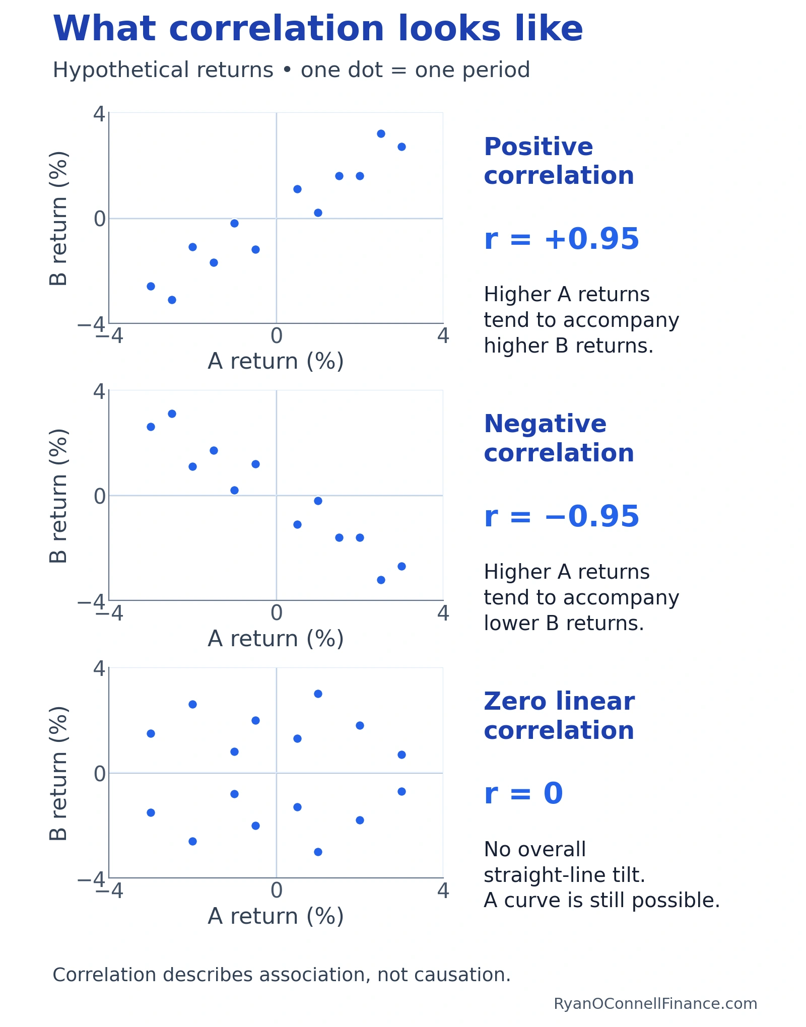
These interpretations concern straight-line association.[1]
For strength, compare absolute values: −0.8 is stronger than +0.4.
The negative sign changes the direction. Labels such as weak, moderate, and strong
need context; the coefficient and scatterplot are more informative than a label
alone.[5]
How the Pearson Correlation Formula Works
Start by expressing each observation relative to its own series’ mean and
sample standard deviation.
The resulting z-score says how many standard deviations the observation
lies above or below its mean.
zy,i = (yi − ȳ) / sy
Here, x̄ and ȳ are the two means; sx and sy are
sample standard deviations from the same paired sample; and n counts the pairs.
The n − 1 denominator matches the use of sample standard deviations in these
z-scores. The calculation needs at least two pairs and variation in each
series.[2]
When both values are above their respective means, their z-scores multiply to
a positive number. Two below-average values also give a positive product.
Opposite-signed deviations give a negative product. The formula balances these
products on a unitless scale. “Above average” and “below average” refer to each
series’ own mean, which need not be zero.
Correlation Example: Five Hypothetical Days
Suppose Coca-Cola and PepsiCo had the following invented daily price
returns. These are teaching inputs, not either stock’s actual performance.
Five observations keep the arithmetic visible; they are not a recommendation for
estimating an investment relationship.
| Day | Coca-Cola return | PepsiCo return | Coca-Cola z | PepsiCo z | Product |
|---|---|---|---|---|---|
| 1 | −1% | −1% | −1 | −1 | 1 |
| 2 | −1% | 0% | −1 | 0 | 0 |
| 3 | 0% | −1% | 0 | −1 | 0 |
| 4 | +1% | +1% | 1 | 1 | 1 |
| 5 | +1% | +1% | 1 | 1 | 1 |
1. Find the means. Coca-Cola:
(−1 − 1 + 0 + 1 + 1) / 5 = 0%.
PepsiCo: (−1 + 0 − 1 + 1 + 1) / 5 = 0%.
2. Find the sample standard deviations. Using the return numbers
in percentage-point units, each series’ squared deviations sum to 4.
Each sample standard deviation is [4 / (5 − 1)]1/2 = 1
percentage point. Dividing each deviation by 1 gives the z-scores in the table.
3. Add the paired products and divide.
r = (1 + 0 + 0 + 1 + 1) / (5 − 1) = 3 / 4 = 0.75.
The hypothetical sample has positive linear association. Its correlation of
0.75 summarizes the paired standardized deviations; it is not a count of
same-direction trading days or a forecast of either stock’s return.
Correlation vs. a Regression Slope
Pearson Correlation
- Describes linear direction and strength.
- Has no units and stays between −1 and +1.
- Gives the same r if you swap the two variables.
Regression Slope
- Describes how a fitted outcome changes as an explanatory variable changes.
- Uses outcome units per unit of the explanatory variable.
- Depends on which variable is treated as the outcome.
A correlation alone does not supply an equation for predicting returns.
See simple linear regression for slopes,
intercepts, and model assumptions.[2]
For the relationship with covariance and its use in portfolio calculations,
read the separate guide to correlation vs covariance.
How to Calculate and Check Correlation
- Define the question. Choose the variables, return measure,
frequency, and period before inspecting the result. - Match the observations. Pair each return with the other
asset’s return for the same interval. Handle missing pairs consistently. - Inspect the scatterplot. Look for curvature, unusual
observations, and differences between groups that one coefficient could hide. - Calculate and report the context. Record r alongside the
number of pairs, dates, and data definitions. A result without those inputs
is difficult to interpret or reproduce.
A spreadsheet or statistical package can calculate r directly from matched data.
If you already have covariance and the two standard deviations, the existing
calculator below computes correlation from those summary inputs.
Common Mistakes
- Reading r as a percentage. A correlation of 0.75 does not
mean a 75% chance of a gain or 75% same-direction days. - Treating a negative sign as weak. Strength depends on the
magnitude; −0.8 has more linear strength than +0.4. - Confusing price trends with return co-movement. When the
question concerns daily investment performance, analyze matching daily returns. - Mixing dates or frequencies. Today’s return paired with
yesterday’s return answers a different question from same-day correlation. - Reporting a coefficient without its sample. Include the
period and number of pairs instead of implying the result applies everywhere.
Limitations of Correlation
A Curved Relationship Can Have Zero Correlation
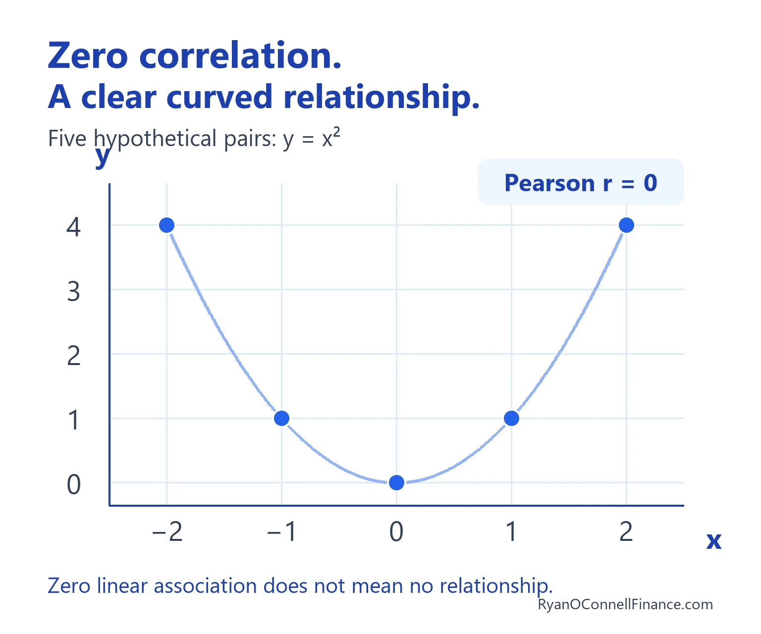
Consider invented values x = −2, −1, 0, 1, 2 and
y = 4, 1, 0, 1, 4. They follow the exact relationship
y = x2. Yet Pearson’s r is zero.
The means are 0 and 2. The centered cross-products sum to
(−2 × 2) + (−1 × −1) + (0 × −2) +
(1 × −1) + (2 × 2) = −4 + 1 + 0 − 1 + 4 = 0.
Both variables vary, so dividing this zero sum by the nonzero standardization factor
gives r = 0. A scatterplot reveals the U shape that the coefficient misses.[4]
Unusual Observations Can Change the Result
A point far from the rest can strengthen or weaken r, depending on where it
falls.[4]
Check for errors, then investigate valid unusual observations. If you compare results
with and without a point, explain why and recalculate the means and standard deviations
for each sample. Removing a real observation simply to obtain a preferred result
misrepresents the evidence.
Correlation Cannot Establish Cause or Guarantee Future Behavior
Even a high correlation between Coca-Cola and PepsiCo returns would not establish
that one company’s gains caused the other’s. Shared market or industry news could
influence both. Establishing causation requires evidence beyond the correlation
itself.[3]
The calculated r also describes the observations you supplied. Changing the
period or return frequency changes those observations and can change the result.
A historical estimate by itself does not establish how the relationship will
behave in a future period.
Frequently Asked Questions
each series’ mean. Counting how often both returns are positive or both
are negative is a different calculation.
same linear strength, with opposite directions. Compare distance from
zero when comparing strength.
and treatment of missing observations. Different inputs can produce
different sample correlations. Compare results calculated on the same basis.
standard deviation of zero, so the formula would divide by zero.
Undefined correlation is different from a valid correlation of zero.
in a series from percentages to decimals rescales its mean and standard
deviation together, leaving each z-score unchanged. Keep units consistent
within each series.
Sources
Primary sources consulted October 29, 2026. The worked returns and U-shaped
dataset are hypothetical; no historical stock correlation is asserted.
- NIST, Dataplot Reference Manual: Correlation, March 18, 1997, description and equation 2-5.
- Penn State Department of Statistics, STAT 200, Lesson 12: Correlation & Simple Linear Regression, sections 12.1, 12.2, 12.3, and 12.5.
- NIST/SEMATECH, Engineering Statistics Handbook: Scatter Plot, definition, diagnostic questions, and causality discussion.
- University of California, Berkeley, SticiGui: Correlation and Association, nonlinear association, outliers, and summary.
- U.S. Environmental Protection Agency, Exploratory Data Analysis: Correlation Analysis, updated February 3, 2026.
- U.S. Securities and Exchange Commission, Investor.gov, Diversification.
Disclaimer
This article is for educational purposes and does not constitute investment advice.
Hypothetical examples explain statistical mechanics and do not describe actual security
performance or predict future returns.
Keep reading
More in Quantitative Finance
-
Standard Deviation in Finance: Volatility Explained
Standard deviation measures the dispersion of investment returns, quantifying how much a stock or portfolio’s performance varies over time.
-
Portfolio Diversification: What It Is, How It Works, and Why It Matters
Learn how portfolio diversification reduces risk, the diversification ratio formula, and practical strategies for building a well-diversified portfolio.
-
Capital Asset Pricing Model (CAPM): Formula and Example
The Capital Asset Pricing Model describes the relationship between systematic risk and expected return, providing a framework for pricing risky assets.