
Volatility Estimation: EWMA and GARCH Models Explained

Table of Contents
The GARCH model is the industry standard for estimating and forecasting financial market volatility. Unlike simple historical measures that treat all past observations equally, conditional volatility models like EWMA and GARCH recognize a fundamental truth about financial markets: volatility changes over time, and recent returns carry more information about current risk than distant ones. This guide covers the full progression — from basic historical variance to the GARCH(1,1) model used by banks, risk managers, and derivatives traders worldwide.
Understanding how to estimate volatility is essential for anyone involved in risk management, option pricing, or portfolio construction. A Value at Risk (VaR) model is only as good as its volatility input. A derivatives trader who misprices volatility will misprice options. This article explains the key models, their formulas, and when to use each one — with a worked example you can follow step by step.
What Is Volatility Estimation?
Volatility measures the magnitude of price fluctuations in a financial asset. Unlike price or return, volatility is not directly observable — it must be estimated from historical return data or inferred from option prices (implied volatility). This article focuses on the first approach: estimating volatility from observed returns.
Conditional volatility models (EWMA, GARCH) recognize that volatility is not constant — it changes over time in predictable ways. Periods of large price swings tend to cluster together, a phenomenon called volatility clustering. These models give more weight to recent observations, producing volatility estimates that adapt to current market conditions.
The distinction between unconditional and conditional volatility is central to this topic. Unconditional volatility is a single long-run average — treat all data equally and compute one number. Conditional volatility changes at each point in time, reflecting the information available up to that moment. For risk management, conditional estimates are far more useful because they capture the current volatility regime.
An important simplification used throughout: for daily returns, the expected return is approximately zero (the daily drift is negligible compared to daily volatility). This means we can use observed returns rt directly in variance formulas without subtracting the mean — a standard convention in volatility modeling.
Simple Historical Volatility
The simplest approach to estimating volatility is to compute the realized variance — the equally weighted average of squared daily returns over a lookback window of n days.
This is the realized variance form under the zero-mean assumption. It differs from the textbook sample variance formula (which uses 1/(n-1) and subtracts the sample mean), but for daily data with hundreds of observations and a near-zero mean, the difference is negligible. To annualize, multiply the daily variance by 252 (trading days per year) and take the square root:
The key limitation: every observation receives equal weight, regardless of how recent it is. A return from six months ago has the same influence as yesterday’s return. Consider the March 2020 COVID crash — the S&P 500 fell over 30% in weeks, then recovered sharply. A 1-year historical volatility estimate would remain elevated for months after markets had calmed, overstating the true current risk. This is the motivation for weighted approaches.
EWMA (Exponentially Weighted Moving Average)
The Exponentially Weighted Moving Average (EWMA) model addresses the equal-weighting problem by assigning exponentially declining weights to past observations. Recent returns matter more; distant returns fade away.
Where λ (lambda) is the decay factor, typically between 0.90 and 0.99. JPMorgan’s RiskMetrics system, introduced in 1994, popularized λ = 0.94 for daily data and λ = 0.97 for monthly data. The weight assigned to an observation k trading days ago is (1 – λ)λk-1, for k ≥ 1. With λ = 0.94, yesterday’s return (k = 1) receives a 6% weight; a return from 30 trading days ago receives about 16.6% of yesterday’s weight.
For a hypothetical comparison, take a 60-trading-day historical window, so each included squared daily return receives the same weight. Compare it with EWMA using λ = 0.94 over its full history. Observation age 1 means yesterday and age 60 means 60 trading days ago; the figure shows those 60 ages without rescaling the EWMA weights.
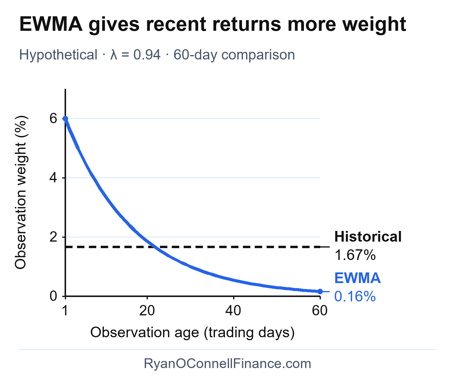
EWMA assigns 6.00% to yesterday’s squared return, versus 1.67% in the 60-day historical estimate. By age 60 its weight is about 0.16%; the remaining 2.44% of EWMA’s total weight lies on observations older than 60 trading days.
EWMA is mathematically equivalent to an IGARCH(1,1) model with ω = 0 and α + β = 1. This means EWMA has no finite unconditional variance and no mean reversion — volatility shocks persist indefinitely in the forecast. This is both a strength (simplicity, responsiveness) and a weakness (no long-run anchor). The GARCH model addresses this limitation.
To illustrate, consider Apple (AAPL) stock with yesterday’s EWMA variance estimate of σn-1² = 0.00025 (1.58% daily vol) and yesterday’s return of rn-1 = -4.5% following an earnings miss. Using λ = 0.94: σn² = 0.94 × 0.00025 + 0.06 × 0.002025 = 0.000235 + 0.000122 = 0.000357, giving σn = 1.89% daily. The single large return immediately increased the volatility estimate from 1.58% to 1.89% — and under EWMA, this elevated level will persist in all future forecasts until offset by smaller returns.
The GARCH(1,1) Model — Formula and Parameters
The Generalized Autoregressive Conditional Heteroskedasticity (GARCH) model, introduced by Tim Bollerslev in 1986, extends EWMA by adding a crucial third component: a constant term ω that pulls volatility back toward a long-run level.
Where ω > 0, α ≥ 0, β ≥ 0, and α + β < 1 (the covariance stationarity condition).
Parameter interpretation:
- α (alpha) — shock sensitivity: how strongly yesterday’s squared return (new information) affects today’s variance estimate. Higher α means volatility reacts more sharply to market surprises.
- β (beta) — persistence: how much of yesterday’s conditional variance carries forward. Higher β means volatility decays slowly after a shock.
- ω (omega) — baseline contribution: ensures variance has a positive floor and drives mean reversion to the long-run level.
The sum α + β is called persistence — it determines how slowly forecast variance converges toward VL after a shock. The variance-shock half-life (trading days for the expected variance gap from VL to halve) is approximately ln(0.5) / ln(α + β). This is the key advantage of GARCH over EWMA: mean reversion. Conditional variance above VL is forecast to decline toward it, while conditional variance below VL is forecast to rise toward it.
The “(1,1)” in GARCH(1,1) refers to 1 lag of the squared return and 1 lag of the conditional variance. This specification is sufficient for the vast majority of financial applications — higher-order models like GARCH(2,1) rarely provide meaningful improvement.
GARCH Model Example
For a hypothetical S&P 500 example, a risk manager uses the following illustrative GARCH(1,1) parameters; these are not fitted market estimates:
- ω = 0.000002
- α = 0.08
- β = 0.90
- Persistence = α + β = 0.98
Yesterday’s estimated daily variance was σn-1² = 0.0004 (corresponding to 2% daily volatility), and yesterday’s return was rn-1 = -3% (a sharp sell-off).
Step 1: Calculate today’s conditional variance:
σn² = 0.000002 + 0.08 × (-0.03)² + 0.90 × 0.0004
= 0.000002 + 0.08 × 0.0009 + 0.90 × 0.0004
= 0.000002 + 0.000072 + 0.000360 = 0.000434
Step 2: Convert to daily volatility:
σn = √0.000434 = 2.08% daily (≈ 33.0% annualized)
Step 3: Compare to long-run volatility:
VL = 0.000002 / (1 – 0.98) = 0.0001 → σL = 1.0% daily (≈ 15.9% annualized)
Step 4: Interpret:
Current volatility (2.08% daily) is well above the long-run level (1.0% daily). The -3% return increased the variance estimate from 0.0004 to 0.000434. With persistence of 0.98, the excess-variance half-life is approximately 34 trading days (about 7 weeks): the forecast variance gap above 0.0001 halves over that interval. This does not mean that daily volatility itself falls by half.
Maximum Likelihood Estimation
GARCH parameters (ω, α, β) cannot be calculated with a simple formula — they are estimated using maximum likelihood estimation (MLE). The idea is to find the parameter values that make the observed return data most probable under the assumed model.
There is no closed-form solution — the log-likelihood must be maximized numerically using optimization algorithms (such as Nelder-Mead or BFGS). The process requires initial parameter guesses and convergence criteria. In practice, software handles this automatically: Python’s arch package, R’s rugarch, or MATLAB’s garch function.
A reliable GARCH fit typically requires 500 to 1,000+ daily observations (roughly 2-4 years of trading data). Fewer than 250 observations often produces unstable or unreliable parameter estimates. After fitting, always check standardized residuals (rt / σt) for remaining ARCH effects — if the model is well-specified, these residuals should behave like independent draws. If standardized residuals show excess kurtosis (fat tails), a Student-t distribution may be more appropriate than the Gaussian assumption.
EWMA vs GARCH Model — Key Differences
Both EWMA and GARCH capture volatility clustering, but they differ in fundamental ways that affect when each model is appropriate.
EWMA
- 1 parameter (λ, typically 0.94)
- Minimal calibration — λ typically set to 0.94 (can be optimized)
- IGARCH: no mean reversion
- No finite unconditional variance
- Multi-day forecasts are flat (current vol persists)
- RiskMetrics industry standard
- Best for: 1-day VaR, simplicity, speed
GARCH(1,1)
- 3 parameters (ω, α, β)
- Requires MLE estimation from data
- Covariance-stationary: mean-reverts to VL
- Finite unconditional variance (VL)
- Multi-day forecasts converge toward VL
- Academic and regulatory standard
- Best for: multi-day horizons, term structure, formal risk models
For short-horizon applications like 1-day VaR, EWMA and GARCH often produce similar results. The difference becomes significant for multi-day forecasts — GARCH’s mean reversion produces a declining volatility term structure after a shock, while EWMA forecasts a constant level indefinitely. For risk managers building multi-day or multi-week VaR models, GARCH provides a more realistic volatility path.
Volatility Forecasting
One of the most practical applications of GARCH is multi-step-ahead volatility forecasting. The GARCH model’s mean-reversion property creates a natural term structure of volatility.
GARCH forecasting: Return to the hypothetical S&P 500 example with ω = 0.000002, α = 0.08, β = 0.90, and a current one-day variance estimate of 0.000434. Let k count additional trading days beyond this current estimate. Holding the parameters fixed and averaging over future returns, the expected daily variance is VL + (α + β)k(0.000434 – VL), where VL = 0.0001. It approaches this long-run level as k increases; starting below that level would instead produce a rising forecast.
EWMA forecasting: For this comparison, start EWMA from the same daily variance of 0.000434 (2.08% daily volatility). With no new observations, its expected daily variance stays at this starting level because it has no long-run anchor. The figure compares the two forecasts over 150 additional trading days and marks GARCH’s long-run variance.
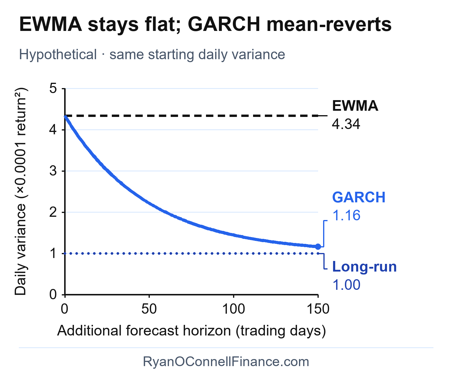
After about 34.3 additional trading days, GARCH’s expected variance gap above 0.0001 has fallen by half: forecast variance is about 0.000267, corresponding to daily volatility of 1.63%. EWMA remains at 0.000434 (2.08% daily volatility). These are forecasts for individual days, rather than variance accumulated over the entire holding period.
This forecasting behavior directly affects risk models. Parametric VaR scales the volatility input across the holding period. Using EWMA for a 10-day VaR will produce a higher estimate (during stressed periods) than GARCH, because GARCH predicts the volatility will partially revert during those 10 days. The choice of model can meaningfully impact capital requirements and risk limits.
Common Mistakes with GARCH Models
Volatility estimation involves statistical complexity that creates several common pitfalls. Avoiding these mistakes is essential for reliable risk management.
1. Using simple historical volatility for risk management. Equally weighted variance ignores volatility clustering — the most important stylized fact of financial returns. After a market shock, simple historical volatility is slow to react (if the lookback window is long) or noisy (if the window is short). Conditional models like EWMA and GARCH are designed specifically for this problem.
2. Blindly using λ = 0.94 without validation. JPMorgan’s RiskMetrics default was calibrated for a broad set of assets in the 1990s. It may not be optimal for all asset classes, time periods, or market regimes. Validate the decay factor against your specific data or use GARCH to estimate the effective weighting from the data itself.
3. Ignoring mean reversion for long-horizon forecasts. Using an EWMA-based volatility estimate for a 30-day or 90-day risk horizon implicitly assumes volatility stays at its current level indefinitely. If volatility is elevated after a crisis, this overstates risk; if depressed during calm markets, it understates risk. GARCH’s mean reversion provides more realistic multi-day forecasts.
4. Estimating GARCH with too few data points. Reliable MLE estimation requires at least 500 daily observations (~2 years). With fewer data points, parameter estimates become unstable and can produce misleading results. The long-run variance VL is especially sensitive to sample size.
5. Confusing conditional and implied volatility. GARCH estimates conditional volatility from historical return data — it is backward-looking. Implied volatility is extracted from option prices and reflects the market’s forward-looking expectation. These two measures serve different purposes and often diverge, especially during market stress.
6. Failing to validate model residuals. Fitting a GARCH model is not the final step. Always check standardized residuals for remaining ARCH effects (using Ljung-Box tests on squared residuals). If the model is well-specified, residuals should be approximately independent. Backtest any VaR model built on GARCH output against realized returns.
7. Assuming normally distributed errors when tails are heavy. Financial returns typically exhibit excess kurtosis — extreme events occur more frequently than a normal distribution predicts. Using Gaussian GARCH when returns have fat tails will underestimate tail risk. Consider Student-t or skewed-t innovations when standardized residuals show excess kurtosis.
GARCH Model Limitations
GARCH(1,1) treats positive and negative returns of the same magnitude identically — a +3% return and a -3% return produce the same volatility update. In equity markets, this is unrealistic: negative returns typically increase volatility more than positive returns of equal size (the leverage effect). Asymmetric models like EGARCH and GJR-GARCH address this limitation.
Leverage effect not captured. The asymmetric response of volatility to negative versus positive returns is well-documented in equity markets. After sharp declines, volatility tends to spike more than it would after an equally large rally. Extensions such as EGARCH (Nelson, 1991) and GJR-GARCH (Glosten, Jagannathan, and Runkle, 1993) add a leverage term to capture this asymmetry. For equity applications, these models often provide a better fit than standard GARCH(1,1).
Parameter sensitivity to sample period. GARCH parameters estimated over a calm period (e.g., 2017) can differ significantly from those estimated over a volatile period (e.g., 2008-2009). This sensitivity means the long-run variance VL itself is an estimate, not a fixed constant. Practitioners should re-estimate parameters periodically and conduct sensitivity analysis.
Distributional assumptions affect tail risk. The standard Gaussian GARCH model underestimates the probability of extreme returns. Using a Student-t distribution for innovations improves tail fit but introduces an additional parameter (degrees of freedom) that must be estimated. The choice of distribution directly affects risk measures like Value at Risk and parametric VaR at high confidence levels.
Higher-order models add complexity with marginal benefit. GARCH(2,1) or GARCH(1,2) models add more lag terms, but empirical evidence consistently shows that GARCH(1,1) captures the vast majority of conditional variance dynamics. The additional parameters rarely justify the added estimation complexity.
Despite these limitations, GARCH(1,1) remains the workhorse of volatility estimation. Its combination of parsimony (three parameters), mean reversion, and strong empirical performance makes it the default choice for practitioners across risk management, derivatives pricing, and portfolio construction. Volatility estimation also plays a role beyond trading desks — real options analysis requires estimating project cash flow uncertainty, and employee stock option valuation under FASB ASC 718 depends on reliable volatility inputs.
Frequently Asked Questions
Disclaimer
This article is for educational and informational purposes only and does not constitute investment or financial advice. The GARCH parameters and example calculations are illustrative and do not represent actual fitted model parameters for any specific security. Volatility models involve statistical assumptions that may not hold in all market conditions. Always conduct your own analysis and consult qualified financial professionals before making risk management or investment decisions.
Keep reading
Next in this series
Part 2 of 3 in Volatility Modeling
Historical Volatility: Parkinson, Garman-Klass & Rogers-SatchellMore in Options & Derivatives
-
Call Options: Buying and Selling Calls Explained
Complete guide to call options — how they work, buying vs selling calls, payoff diagrams, and when to use call options in your trading strategy.
-
Put Options: Buying and Selling Puts Explained
Complete guide to put options — how they work, buying vs selling puts, payoff diagrams, hedging applications, and when to use put options.
-
Option Greeks: The Complete Beginner’s Guide
Complete guide to the five option Greeks — delta, gamma, theta, vega, and rho — what they measure, how they interact, and how to use them for options analysis.


