The Market for Loanable Funds

By Ryan O'Connell, CFA, FRM Published March 10, 2026

The loanable funds market is the fundamental model economists use to explain how interest rates are determined in the long run. Whether you are analyzing why mortgage rates rise after a government spending increase, evaluating how tax policy affects business investment, or studying for an economics exam, the loanable funds framework connects saving, investment, and interest rate movements in a single intuitive model. This guide covers the complete model: the saving-investment identity, what drives supply and demand for funds, how the equilibrium interest rate is determined, and how government policy shifts the market.

What Is the Loanable Funds Market?

The loanable funds market is a simplified model of the financial system that shows how saving (the supply of funds) and investment (the demand for funds) interact to determine the real interest rate. In this model, all saving flows into a single market where borrowers compete for those funds.

The model treats the entire financial system — banks, bond markets, stock markets, and other intermediaries — as a single market where savers supply funds and borrowers demand them. While this is a simplification, it captures the essential mechanism: interest rates coordinate the economy’s saving and investment decisions.

The Loanable Funds Formula

The loanable funds model rests on a fundamental identity from national income accounting. In a closed economy (one without international trade or capital flows), every dollar of output is either consumed, invested, or purchased by the government:

National saving has two components — what households save and what the government saves:

Where Y = national income (GDP), T = taxes, C = consumption, and G = government purchases. When T > G, the government runs a budget surplus and public saving is positive. When G > T, it runs a budget deficit and public saving is negative. Holding the private-saving schedule unchanged, higher public saving shifts national saving right and lower public saving shifts it left.

Supply and Demand for Loanable Funds

The loanable funds market plots planned national saving as supply and planned investment as demand at each real interest rate. However, in this market the “price” is the real interest rate — the inflation-adjusted return on saving and the inflation-adjusted cost of borrowing.

Supply of Loanable Funds

The supply of loanable funds comes from national saving — both private saving by households and public saving by the government. The supply curve slopes upward because higher real interest rates make saving more attractive. When the return on saving increases, households are willing to forgo more current consumption in exchange for greater future purchasing power.

Demand for Loanable Funds

The demand for loanable funds comes from firms and households that want to borrow to invest. Firms borrow to purchase capital equipment, build factories, and fund research. Households borrow to buy homes. The demand curve slopes downward because higher real interest rates make borrowing more expensive, causing fewer investment projects to be profitable. At lower rates, more projects clear the hurdle rate and firms borrow more.

Equilibrium in the Loanable Funds Market

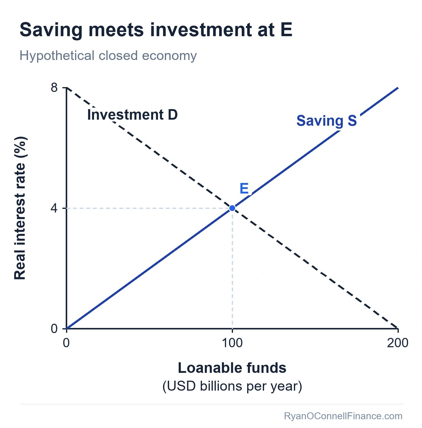
As the diagram above shows, the real interest rate adjusts until planned saving equals planned investment. This equilibrium between plans is distinct from the accounting identity S = I, which holds for recorded outcomes even away from planned equilibrium because investment includes unintended inventories. In the hypothetical diagram, saving and investment both equal USD 100 billion per year at a 4% real interest rate.

If the real interest rate is above equilibrium, planned saving exceeds planned investment — there is a surplus of loanable funds. Lenders compete for borrowers by accepting lower rates, pushing the interest rate down. If the real interest rate is below equilibrium, planned investment exceeds planned saving — there is a shortage. Borrowers compete for funds by offering higher rates, pushing the interest rate up.

This equilibrating process ensures that the economy’s scarce saving is allocated to the investment projects that offer the highest returns. The interest rate serves as the price signal that coordinates millions of individual saving and investment decisions across the economy. This capital accumulation — the conversion of saving into productive investment — is a key driver of long-run economic growth.

Loanable Funds Market Example

Example 1: The Economic Recovery Tax Act of 1981

The Economic Recovery Tax Act of 1981 (ERTA) introduced the Accelerated Cost Recovery System (ACRS), which allowed businesses to depreciate capital assets much faster — effectively subsidizing investment spending. This is a textbook demand-side shift in the loanable funds market.

The faster depreciation made capital purchases cheaper for firms, increasing the quantity of investment demanded at every interest rate. In the loanable funds framework, the demand curve shifts to the right. The predicted result: higher real interest rates and higher quantities of saving and investment.

To illustrate this channel rather than estimate ERTA’s historical effects, increase investment demand in the earlier hypothetical market while holding the saving curve fixed.

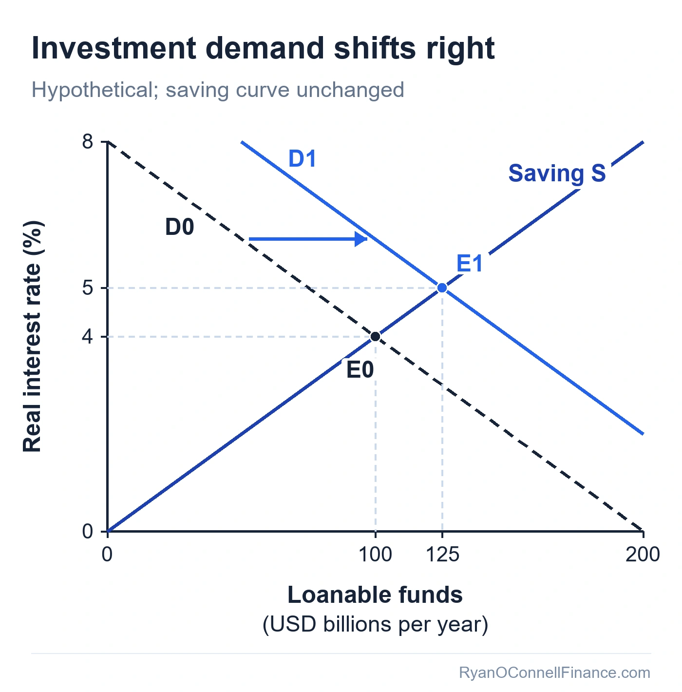
At E1, the real rate is 5% and investment is USD 125 billion per year, up from 4% and USD 100 billion at E0. Saving rises through a movement along the unchanged supply curve. These illustrative values are not an estimate of ERTA’s historical effects; actual early-1980s outcomes also reflected Federal Reserve policy, the business cycle, and budget deficits.

The same logic works in reverse for saving incentives. Tax-advantaged retirement accounts (such as expanded IRA contribution limits) can encourage private saving, but some contributions may relocate existing savings and the tax benefit can reduce public saving. If national saving increases at each rate, supply shifts right; with investment demand unchanged, the model predicts lower real rates and higher investment.

Budget Deficits and the Loanable Funds Market

When the government runs a budget deficit (G > T), public saving turns negative. In this closed-economy comparison, hold the private-saving schedule and investment-demand schedule unchanged. Lower public saving then reduces planned national saving at every rate, shifting supply left. The new equilibrium has a higher real rate and lower private investment.

This mechanism is called crowding out — government borrowing absorbs funds that would otherwise finance private investment, raising borrowing costs for firms and households.

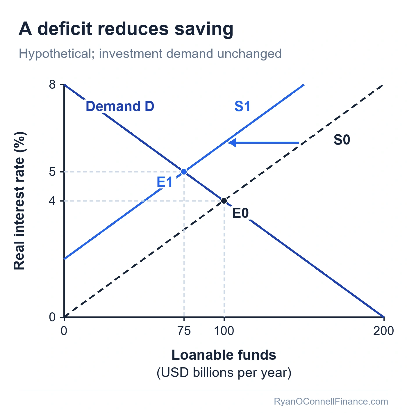
At E1, the real interest rate rises from 4% to 5% and private investment falls from USD 100 billion to USD 75 billion per year. The deficit shifts the saving curve; the higher rate then causes a movement along the unchanged investment-demand curve.

For a full analysis of the crowding out mechanism, including partial crowding out and the Ricardian equivalence debate, see our guide on the crowding out effect. For a broader discussion of long-run fiscal sustainability, see national debt economics.

Loanable Funds Market vs Money Market

The loanable funds market and the money market are two distinct models that explain interest rate determination over different time horizons. Understanding which model applies in which context is essential for macroeconomic analysis.

The key distinction is time horizon. The loanable funds market explains long-run interest rate determination through saving and investment flows. The money market explains short-run interest rate determination through the supply and demand for money. Fiscal policy (taxes and government spending) primarily affects the loanable funds market, while monetary policy (central bank actions) primarily affects the money market. For a deeper look at the money market model, see our guide on money supply and demand.

Common Mistakes

1. Confusing the loanable funds market with the money market. These are two different models that determine two different interest rates. The loanable funds market determines the real interest rate through saving and investment. The money market determines the nominal interest rate through money supply and demand. They answer different questions about different time horizons.

2. Using nominal instead of real interest rates. The vertical axis of the loanable funds diagram is the real interest rate, not the nominal rate. Savers and borrowers make decisions based on inflation-adjusted returns. Plotting the nominal rate confuses the analysis because it conflates changes in inflation with changes in the real cost of borrowing.

3. Mixing conventions for government borrowing. This article uses national saving as supply and private investment as demand. Holding the private-saving schedule unchanged, a larger deficit reduces national saving and shifts supply left. An alternative convention uses private saving as supply and includes government borrowing in demand, so the deficit shifts demand right. Both conventions can describe crowding out; do not count the same deficit on both sides.

4. Applying the closed-economy S = I identity to open economies. The identity S = I holds only in a closed economy. In an open economy with international capital flows, the correct identity is S = I + NCO, where NCO is net capital outflow — the net flow of domestic funds invested abroad. By the balance of payments identity, NCO equals net exports (NX). Foreign capital inflows can supplement domestic saving, which is why the United States has been able to sustain large budget deficits while still funding substantial investment — foreign savers help fill the gap.

Limitations of the Loanable Funds Model

1. Closed-economy assumption. The basic model assumes no international capital flows. In reality, most economies are open, and foreign capital can offset domestic saving shortfalls. The United States has run persistent current account deficits financed by foreign saving for decades — a pattern the closed-economy model cannot explain without modification.

2. Single interest rate. The model assumes a single interest rate equilibrates the market. In practice, there are many interest rates that vary by maturity, credit risk, liquidity, and tax treatment. The yield on a 10-year Treasury bond differs substantially from a 30-year mortgage rate or a corporate bond yield. The model abstracts from this term structure complexity.

3. Assumes flexible interest rates. The model assumes the real interest rate adjusts freely to clear the market. In practice, central banks set short-term nominal interest rates, and various institutional frictions — such as interest rate floors, credit rationing, and regulatory constraints — can prevent real rates from adjusting smoothly to their equilibrium level.