
Logit & Probit Models: Binary Dependent Variables in Regression

Table of Contents
When a bank evaluates a loan application, the outcome is binary: default or no default. An analyst might be tempted to use ordinary least squares to predict this 0/1 outcome, but OLS can produce predicted “probabilities” below zero or above one — nonsensical results for a probability model. The logit model solves this problem by mapping the linear predictor through the logistic cumulative distribution function (CDF), constraining all predicted probabilities to the interval (0, 1). The closely related probit model uses the standard normal CDF instead. Both are estimated by maximum likelihood and have become the standard tools for modeling binary dependent variables in finance and economics. This guide covers the logit and probit specifications, maximum likelihood estimation, how to interpret coefficients through marginal effects and odds ratios, and when to choose logit versus probit versus the linear probability model.
New to the topic? Start with logistic regression explained through scores, odds and prediction cutoffs, then use this guide to compare logit and probit in more depth.
The Problem with OLS for Binary Outcomes
When the dependent variable takes only the values 0 and 1, applying OLS produces the linear probability model (LPM). The LPM interprets the fitted values as probabilities: P̂(Y = 1 | X) = β̂0 + β̂1X1 + … + β̂kXk. While simple and easy to interpret, the LPM has three fundamental limitations for binary outcomes:
- Predicted probabilities outside [0, 1]. Nothing prevents the linear function from producing fitted values of −0.15 or 1.30 — values that have no meaning as probabilities. In credit scoring with extreme borrower profiles, this occurs routinely.
- Inherent heteroskedasticity. Because Var(Y | X) = P(X)[1 − P(X)], the error variance depends on X by construction whenever the slope coefficients are nonzero. Standard errors require robust corrections at minimum.
- Constant marginal effects are unrealistic. The LPM assumes a 1-unit increase in credit score has the same effect on default probability whether the borrower starts at 5% or 50% risk. In reality, marginal effects should diminish near the boundaries.
For observations with predicted probabilities between roughly 0.2 and 0.8, the LPM often agrees closely with logit and probit. Its simplicity makes it useful for quick analysis and difference-in-differences designs. The limitations become severe only when predicted probabilities approach 0 or 1. For a full treatment, see our guide on the linear probability model.
The Logit Model (Logistic Regression)
The logit model (logistic regression) models the probability of a binary outcome by passing the linear index β0 + β1X1 + … + βkXk through the logistic CDF. This ensures that all predicted probabilities lie strictly between 0 and 1, regardless of the values of the independent variables.
Where:
- P(Y = 1 | X) — the predicted probability that the binary outcome equals 1, given the values of the independent variables
- Y — the binary dependent variable (0 or 1)
- β0 — the intercept
- β1 … βk — the slope coefficients for each independent variable
- X1 … Xk — the independent (explanatory) variables
- exp(·) — the exponential function
The logistic function is symmetric around zero: when the linear index equals zero, the predicted probability is exactly 0.5. As the index increases toward positive infinity, the probability approaches 1; as it decreases toward negative infinity, the probability approaches 0. This S-shaped curve naturally captures diminishing marginal effects near the boundaries.
For a constructed comparison, call the linear index z and vary it from −4 to 4. Compare the logit probability 1 / [1 + exp(−z)] with the straight-line rule 0.5 + 0.25z. These rules have the same probability and slope at z = 0; the straight line is an illustrative LPM specification, not an estimate from borrower data.
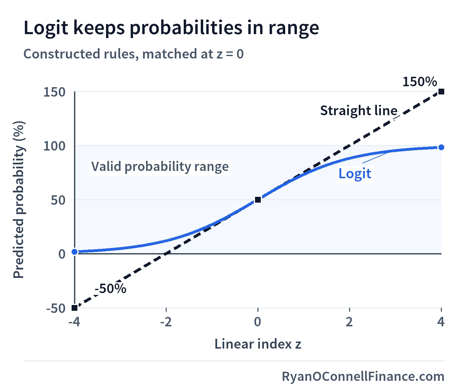
At z = −4, the straight line gives −50%, while logit gives about 1.8%; at z = 4, the values are 150% and about 98.2%. Matching the center does not make the straight line a valid probability rule in the tails.
The logit model can be equivalently expressed through the log-odds (logit) transformation, which linearizes the relationship:
Where:
- P — the predicted probability P(Y = 1 | X)
- P / (1 − P) — the odds of Y = 1 (the ratio of the probability of the event to the probability of the non-event)
- log[P / (1 − P)] — the log-odds (the natural logarithm of the odds), also called the logit
This leads to a powerful interpretation: exponentiating a coefficient gives the odds ratio. If β1 = 0.045, then exp(0.045) = 1.046, meaning a one-unit increase in X1 multiplies the odds of Y = 1 by 1.046 (a 4.6% increase in the odds), holding all other variables constant.
The logit model also has a latent variable interpretation: an unobserved continuous variable y* = β0 + βX + e determines the binary outcome, with Y = 1 when y* > 0. In the logit model, the error term e follows a logistic distribution (mean 0, variance π²/3).
The Probit Model
The probit model replaces the logistic CDF with the standard normal CDF, denoted Φ(·):
Where:
- Φ(·) — the cumulative distribution function (CDF) of the standard normal distribution, which maps any real number to a probability between 0 and 1
In the latent variable framework, the probit model assumes the error follows a standard normal distribution (mean 0, variance 1) rather than a logistic distribution. Because the standard normal has a smaller variance than the logistic distribution (π²/3 ≈ 3.29), probit coefficients are systematically smaller: logit coefficients are approximately 1.6 times probit coefficients. This scaling difference is mechanical — it does not reflect a substantive disagreement between the models.
In practice, logit and probit produce nearly identical predicted probabilities and marginal effects. The logit model has slightly heavier tails, but the difference is rarely meaningful in applied work.
In applied finance, logit is more common because credit risk analysts use odds ratios in scorecard development and coefficient interpretation, making logit the natural choice in the industry. In academic econometrics, probit appears slightly more often because the normal distribution connects naturally to the rest of the statistical theory. In most applications, results are functionally interchangeable.
Maximum Likelihood Estimation
Because the logit and probit models are nonlinear in the parameters, OLS cannot be used. Instead, both models are estimated by maximum likelihood estimation (MLE), which finds the parameter values that make the observed data most probable.
MLE chooses the coefficient vector β that maximizes the likelihood of observing the actual sample outcomes (the observed pattern of 0s and 1s). For binary data with a Bernoulli distribution, the log-likelihood has a clean, well-behaved form that can be maximized numerically.
For each observation i, the contribution to the likelihood is P(Xi)yi × [1 − P(Xi)](1 − yi). Taking the logarithm and summing across all n observations gives the log-likelihood:
Where:
- ln L — the log-likelihood (the natural logarithm of the total likelihood of the observed data)
- yi — the observed binary outcome for observation i (0 or 1)
- P(Xi) — the predicted probability of Y = 1 for observation i, given its covariate values
- n — the number of observations in the sample
There is no closed-form solution — the computer uses iterative numerical methods to find the maximum. Under standard regularity conditions, the MLE is consistent, asymptotically normal, and asymptotically efficient. Standard errors are computed from the inverse of the Hessian matrix (the matrix of second derivatives of the log-likelihood).
To see the objective in a simple hypothetical case, suppose 10 independent loans are observed over one year and exactly 2 default. In an intercept-only model, every loan has the same candidate default probability p. Hold the 10 observed outcomes fixed and vary p: the likelihood of their specific outcome pattern is p2(1 − p)8. The figure divides each likelihood by its maximum, so a relative likelihood of 1 marks the best fit.
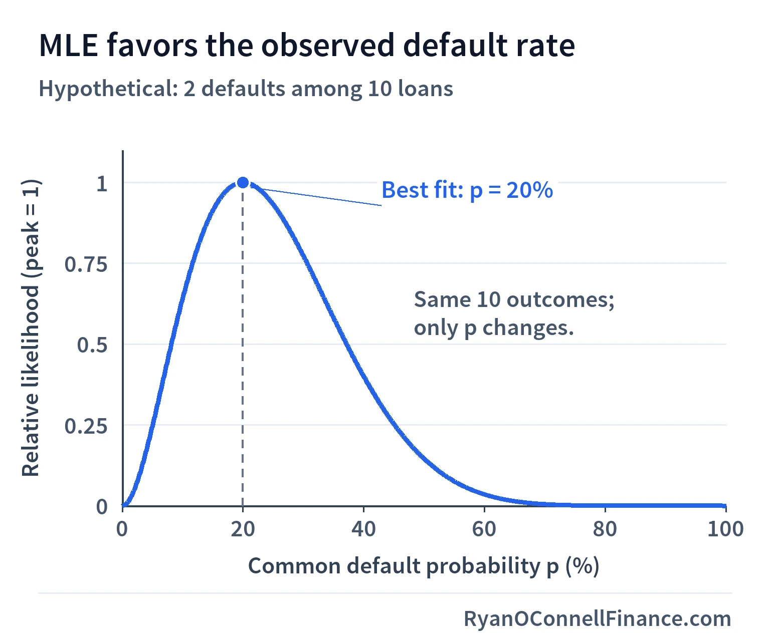
The maximum occurs at p = 20%, equal to 2 defaults divided by 10 loans. Maximizing the log-likelihood gives the same answer because taking logs preserves the ordering. With borrower-level predictors, probabilities can differ across loans and the numerical algorithm adjusts the coefficients jointly.
For testing multiple restrictions simultaneously (the logit/probit analog of the F-test in OLS), the Likelihood Ratio (LR) test compares the log-likelihoods of the restricted and unrestricted models: LR = −2(ln Lr − ln Lur) ~ χ²q, where q is the number of restrictions. For the OLS version of multiple hypothesis testing, see our guide on hypothesis testing in regression.
Model fit is assessed with McFadden’s pseudo R-squared: 1 − (ln Lfull / ln Lnull), where the null model includes only an intercept. As a rough heuristic, pseudo R-squared values of 0.2 to 0.4 are often seen in well-fitting binary models, though the appropriate range depends on the application and data. The percent correctly predicted — the share of observations where the predicted probability correctly classifies Y at a 0.5 threshold — provides an intuitive but crude alternative. However, this metric depends heavily on the chosen cutoff and can be misleading with imbalanced samples: in a loan portfolio where only 5% of borrowers default, a model that predicts “no default” for everyone achieves 95% accuracy while being completely uninformative.
Interpreting Logit and Probit Coefficients
A logit coefficient of −0.008 does not mean the probability decreases by 0.008. In logit and probit models, the marginal effect of any variable depends on the values of all regressors through the nonlinear link function. You must compute marginal effects explicitly — the raw coefficients only indicate the direction and relative magnitude of effects.
The partial effect (marginal effect) of a continuous variable xj on the predicted probability is:
Where:
- ∂P / ∂xj — the marginal effect of variable xj on the predicted probability
- g(·) — the density function of the link distribution: the logistic density g(z) = P(1 − P) for logit, or the standard normal density φ(z) for probit
- β0 + βX — the linear index (the linear combination of all regressors and their coefficients)
- βj — the estimated coefficient on variable xj
The scale factor g(z) is always positive, so the marginal effect has the same sign as βj. Because the marginal effect varies with X, two standard summary measures are used:
- Marginal Effect at the Mean (MEM): Evaluate the partial effect at the sample mean values of all regressors. Simple to compute, but the “average borrower” may not be representative of any actual borrower.
- Average Marginal Effect (AME): Compute the partial effect for every observation in the sample, then average. This uses the full distribution of X values and is generally preferred by applied researchers.
For logit, the maximum scale factor is 0.25 (when the predicted probability equals 0.5), so the largest possible marginal effect for any variable is 0.25 × βj. For probit, the maximum scale factor is approximately 0.40 (at z = 0).
The derivative formula above applies only to continuous regressors. For binary (indicator) variables — such as “has collateral” (0 or 1) — compute the discrete change in predicted probability: ΔP = P(Y = 1 | d = 1, X) − P(Y = 1 | d = 0, X), holding all other variables at the same values. This gives the exact effect of switching the indicator from 0 to 1, rather than an approximation based on the derivative.
In this hypothetical one-year example, a bank models loan default (Y = 1 if default during the year, 0 otherwise) using credit score, debt-to-income ratio (DTI), and a collateral indicator (1 if collateral is present, 0 otherwise). The illustrative logit coefficients are:
| Variable | Coefficient | Odds Ratio |
|---|---|---|
| Intercept | 3.200 | — |
| Credit Score | −0.008 | 0.992 |
| DTI (%) | 0.045 | 1.046 |
| Has Collateral (0/1) | −0.620 | 0.538 |
Hold DTI fixed at 35% and use the same one-year default horizon for all profiles. Borrower A has a credit score of 700 and Borrower B has a score of 750; both initially have no collateral. Vary the score from 500 to 850, using the table’s coefficients throughout, and compare collateral = 0 with collateral = 1 at each score. Points beyond the worked scores of 700 and 750 are additional hypothetical model evaluations.
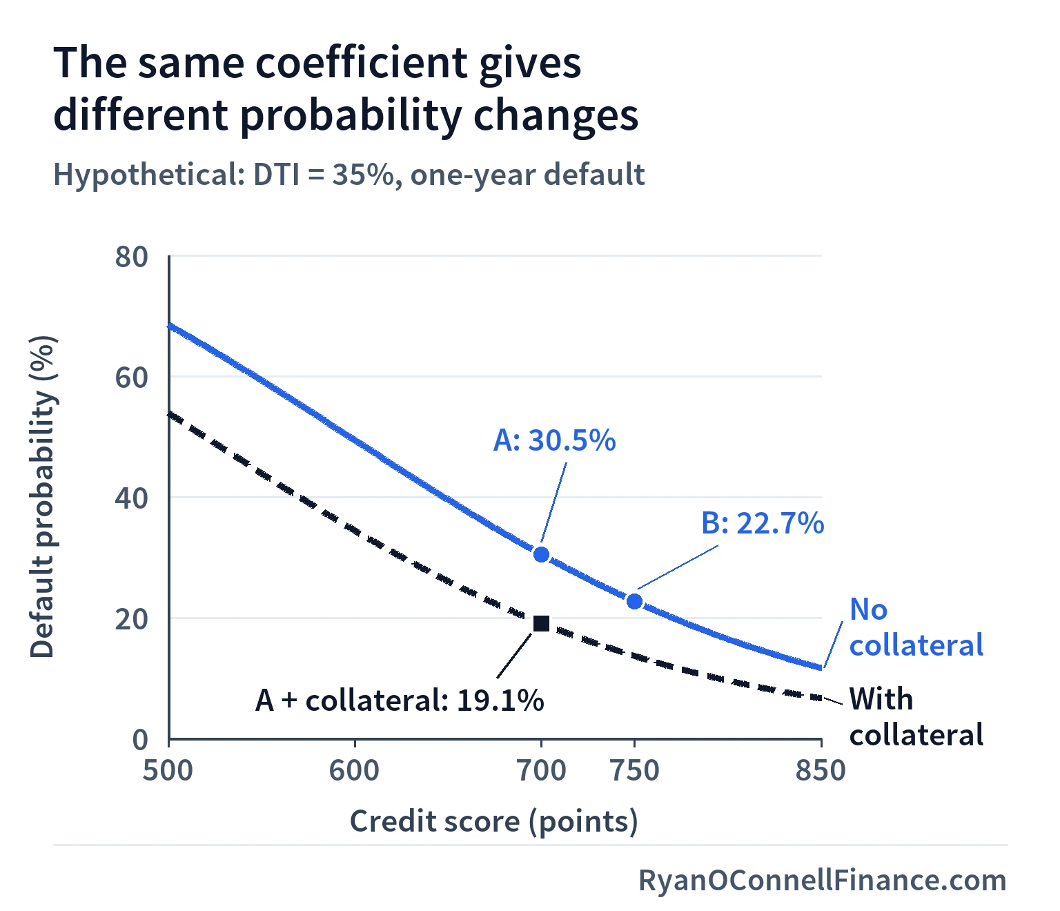
The same 50-point score increase lowers risk by about 9.8 percentage points from 600 to 650, but by 7.8 points from 700 to 750. For the fixed score-700 profile, switching collateral on lowers risk from 30.5% to 19.1%. The calculations below separate the continuous score effect from the exact binary switch.
Borrower A: Credit Score = 700, DTI = 35%, collateral = 0
- Linear index: Xβ = 3.200 + (−0.008)(700) + (0.045)(35) = 3.200 − 5.600 + 1.575 = −0.825
- Predicted probability: P = exp(−0.825) / [1 + exp(−0.825)] = 0.4385 / 1.4385 = 0.305 (30.5%)
- Marginal effect of credit score: 0.305 × (1 − 0.305) × (−0.008) = −0.0017 — a 1-point increase in credit score reduces default probability by 0.17 percentage points
- Odds ratio for DTI: exp(0.045) = 1.046 — a 1-percentage-point increase in DTI multiplies the odds of default by 1.046 (4.6% higher odds)
Borrower B: Credit Score = 750, DTI = 35%, collateral = 0 (same DTI and collateral status, higher credit score)
- Linear index: Xβ = 3.200 + (−0.008)(750) + (0.045)(35) = 3.200 − 6.000 + 1.575 = −1.225
- Predicted probability: P = exp(−1.225) / [1 + exp(−1.225)] = 0.2938 / 1.2938 = 0.227 (22.7%)
Discrete change for collateral (binary regressor): For Borrower A’s profile (Score = 700, DTI = 35%), compare collateral = 0 vs. collateral = 1:
- Without collateral: Xβ = −0.825 + (−0.620)(0) = −0.825 → P = 0.305
- With collateral: Xβ = −0.825 + (−0.620)(1) = −1.445 → P = exp(−1.445) / [1 + exp(−1.445)] = 0.191 (19.1%)
- Discrete change, using unrounded probabilities: 0.19077 − 0.30470 = −0.11393 — having collateral reduces default probability by about 11.4 percentage points
Holding DTI constant at 35%, a 50-point credit score improvement (700 → 750) reduces default probability from 30.5% to 22.7% — a 7.8-percentage-point drop. This illustrates the nonlinear nature of the logit model: the marginal effect of credit score is larger at higher baseline risk levels and diminishes as the predicted probability moves away from 0.5. The collateral example shows how binary regressors require a discrete-change approach rather than the derivative formula.
Logit vs. Probit vs. Linear Probability Model
Logit Model
- Link function: Logistic CDF
- Predicted probabilities: Always in (0, 1)
- Coefficients: Log-odds; convert to odds ratios via exp(β)
- Estimation: Maximum likelihood
- Marginal effects: Vary with X; must compute MEM or AME
- Best for: Large samples, boundary probabilities matter, odds ratio interpretation valued
Probit Model
- Link function: Standard normal CDF
- Predicted probabilities: Always in (0, 1)
- Coefficients: Index units; no direct odds ratio interpretation
- Estimation: Maximum likelihood
- Marginal effects: Vary with X; must compute MEM or AME
- Best for: Academic research, latent variable interpretation, normal-distribution-based theory
Linear Probability Model
- Link function: None (identity)
- Predicted probabilities: Can fall below 0 or exceed 1
- Coefficients: Direct marginal effects (constant)
- Estimation: OLS
- Marginal effects: Coefficients ARE marginal effects
- Best for: Quick analysis, interior probabilities, difference-in-differences designs
In practice, all three models produce similar marginal effects when predicted probabilities are well within the (0.2, 0.8) range. The choice matters most at the tails — when modeling events with very high or very low base rates (such as loan defaults, which typically occur in 1–5% of a portfolio), logit and probit provide more reliable probability estimates than the LPM. When comparing logit and probit results, always compare average marginal effects (AMEs), not raw coefficients — the raw coefficients differ by a factor of approximately 1.6 due to the different scale of the underlying distributions, but the AMEs will be nearly identical.
Applications in Finance
Logit and probit models are widely used across financial applications wherever the outcome is naturally binary:
- Credit scoring and probability of default. Banks estimate the probability that a borrower will default on a loan using financial ratios, credit history, and macroeconomic variables as predictors. Logit is the dominant model in the industry due to its odds ratio interpretation. For the full probability of default framework including Basel regulatory requirements, see our guide on credit risk and probability of default.
- Customer churn prediction. Financial services firms model whether a client will close an account (Y = 1) or remain (Y = 0) based on account activity, fee sensitivity, service interactions, and competitor pricing.
- Merger and acquisition prediction. Researchers model whether a target firm will receive a takeover bid as a function of firm size, Tobin’s Q, leverage, free cash flow, and industry concentration.
- Buy/sell signal models. Quantitative analysts predict whether a stock will outperform a benchmark over the next period (Y = 1) or not (Y = 0), using fundamental ratios, technical indicators, and momentum variables as inputs.
A researcher estimates a logit model for takeover bids among S&P 500 firms (Y = 1 if the firm receives a bid). Selected coefficients:
- Leverage: β = 0.82, odds ratio = exp(0.82) = 2.27 — each 1-unit increase in leverage more than doubles the odds of receiving a takeover bid
- Tobin’s Q: β = −0.35, odds ratio = exp(−0.35) = 0.70 — higher-valued firms are less likely targets (30% lower odds per unit of Q)
- log(Assets): β = −0.18, odds ratio = exp(−0.18) = 0.84 — larger firms are harder to acquire
These odds ratios align with the corporate finance intuition that highly leveraged, undervalued, and smaller firms are more attractive acquisition targets.
Common Mistakes
1. Interpreting logit or probit coefficients as marginal effects. A logit coefficient of −0.008 does not mean the probability drops by 0.008. The marginal effect depends on the values of all regressors through the density function g(Xβ). Always report average marginal effects (AME) or marginal effects at the mean (MEM) alongside raw coefficients to convey the economic magnitude of the relationship.
2. Comparing pseudo R-squared to OLS R-squared. McFadden’s pseudo R-squared typically ranges from 0.2 to 0.4 for well-fitting binary models. A pseudo R-squared of 0.25 does not mean the model “only explains 25% of the variation” — it is a fundamentally different metric measured on a different scale. Comparing pseudo R-squared values across logit models is reasonable; comparing them to OLS R-squared values is not.
3. Not reporting marginal effects. Publishing only raw logit coefficients or odds ratios without marginal effects makes it impossible for readers to assess the economic magnitude of each predictor. Marginal effects translate results into probability-scale changes that can be compared across studies and models.
4. Ignoring finite-sample bias and separation. These are related but distinct problems. Finite-sample bias: MLE is a large-sample estimator, so with fewer than roughly 10 events (Y = 1) per estimated parameter, logit and probit coefficients can be substantially biased and standard errors inflated. A common rule of thumb is at least 10 events per predictor. Separation is a different issue: it occurs when a predictor (or combination of predictors) perfectly predicts the outcome for a subset of observations, causing one or more coefficient estimates to diverge toward ±∞. Separation can arise even in moderately large samples if a category has zero events — for example, if no borrower with collateral ever defaults in the sample.
5. Comparing raw coefficients across logit and probit models. Logit coefficients are approximately 1.6 times probit coefficients because the logistic distribution has a larger variance (π²/3 ≈ 3.29) than the standard normal (variance = 1). Comparing magnitudes directly without adjusting for this scale difference is meaningless. Compare marginal effects instead — they will be nearly identical across the two models.
Frequently Asked Questions
Disclaimer
This article is for educational and informational purposes only and does not constitute investment advice. The regression coefficients, predicted probabilities, and marginal effects used in examples are illustrative and may differ based on the data source, sample period, and model specification. Always conduct your own analysis and consult a qualified financial advisor before making investment decisions. Reference: Wooldridge, Jeffrey M. Introductory Econometrics: A Modern Approach, 8th Edition, Cengage, 2025.
Keep reading
Next in this series
Part 15 of 17 in Econometrics: From Regression to Causal Inference
Cointegration, Unit Root Tests & Error Correction ModelsMore in Econometrics
-
What Is Econometrics? Data Types, Causality & the Empirical Process
Econometrics applies statistical methods to economic and financial data to estimate relationships, test theories, and evaluate decisions.
-
Simple Linear Regression: The OLS Method Explained
Learn simple linear regression and the OLS method. Understand the population model, slope and intercept interpretation, R-squared, and key assumptions…
-
Time Series Regression: Trends, Seasonality & Stationarity
Time series regression models dynamic relationships in financial and economic data. Learn what makes time series special, how to handle trends and seasonality…




